Algorithm complexity
Introductory examples
We intuitively understand that the amount of operations required by an algorithm usually depends on the size of input data. Let consider a simple example with an algorithm, often called linear-search, that tries to find the first cell in an array of size \(n\) that contains a given element:
def find(array, element):
  for i in range(len(array)):
    if array[i] == element:
      return i
  return -1
This algorithm takes as input an array of size len(length) and an element.
It browses the array elements from the first to the last one.
If, at iteration i it encounters the value element at the position i of array, it stops and returns the index value i.
If we reach the end of the for loop, meaning that the element is not in the array, it returns the value -1.
Some examples of executions of linear-search:
i1 = find([3,5,6], 3) # i1 = 0
i2 = find([3,5,6], 6) # i2 = 2
i3 = find([3,5,6], 8) # i3 = -1
Pseudocode
Algorithms are usually written in pseudocode. In this course, we will follow the Python syntax for pseudocode. Pseudocode algorithms should be easy to implement in common programming languages such as C, C++, Java, and so we will forbid ourselves from using Python specificities that are not common to other languages (for example dictionaries, list comprehensions, high level functions). We will also avoid using specific libraries (like numpy, pandas, etc.) that are not part of the standard libraries of most programming languages.
In practice we will only use simple Python constructs like loops, conditions, and basic data structures (numbers, lists, strings).
We can see that in the worst case, if the searched element is not in the array, the algorithm has to browse the whole array, and it performs n comparisons.
In other words, in the worst case, the number of operations performed by this algorithm is proportional to the size of the input.
On the other hand, we might get lucky: if the searched element is located in the first cell of the array, we will perform a single comparison.
So, in general, the number of operations depends on the size of the input n.
However, the number of operations for two different inputs with the same size can be different:
we can thus ask ourselves what is the number of operations in the worst case ? In the average case ? In the best case ?
We will often concentrate on the worst case as:
The worst case gives a guaranteed upper bound on the runtime for any input.
The average case analysis requires assuming a probability distribution of the input which is difficult to test in practice.
The best case is often meaningless. For example in linear search, the best case (the searched element is in the first cell of the array) requires a simple comparison, but that doesn’t help us much to understand the algorithm.
Warning
In the following, time complexities are given by default in the worst case.
Amortized complexity
In the chapter about data-structures, we will see a 4-th possibility called amortized complexity, where we consider the average number of operations when an algorithm is called several times on the same data-structure.
When we perform the analysis of an algorithm we usually have to do some assumptions and simplifications on the cost of basic operations. We usually use the RAM (Random Access Machine) model where all the basic operations take a bounded time (this time might be different for different operations, but it does not depend on the size of the input):
simple arithmetic and comparison operations on integers and floating point numbers (+, -, /, *, %, <, <=, ==, …)
random memory access (we can store and read an integer or a float anywhere in memory)
control (if, function call, return…)
Random Access Machine model limitations
The hypothesis of the RAM model may not be verified in practice as bounded time arithmetic operations only exist for numbers that are small enough to be represented by a built-in data type of the processor (int, float, double…).
For large numbers we have to use custom data types (BigNumber, BigInteger, BigDecimal) whose basic arithmetic operations have a runtime complexity that depends on the number of bits needed to represent the numbers.
Math reminder
Here is a quick reminder on some useful mathematical properties. In the following \(a\), \(b\), and \(c\) are positive numbers, and \(n\) is a positive integer:
\(a^b a^c = a^{b+c}\)
\(\frac{1}{a^b} = a^{-b}\)
\((a^b)^c = a^{bc}\)
\(\sqrt{a}=a^{0.5}\)
\(\log(ab)=\log(a) + \log(b)\)
\(\log_c(b) = \frac{\log(b)}{\log(c)}\)
\(\lim_{x\rightarrow \infty}\frac{x^a}{x^b}=0\), if \(b>a\)
\(\lim_{x\rightarrow \infty}\frac{\log^a(x)}{x^b}=0\)
\(1+2+\ldots + n = \frac{n(n+1)}{2}\)
Asymptotic complexity
Complexity analysis is at the heart of algorithm design. In the previous section, we have seen on a simple example that the number of operations done by an algorithm is a function \(f\) of the parameter \(n\) denoting the size of the input problem. Usually, this function \(f\) is increasing: the larger the problem, the more operations we have to do to solve it. In complexity analysis, we want to study at which rate \(f\) growths when \(n\) increases. In other words, we are not interested about small inputs or small variations in the number of operations: we want to know how the algorithm behaves when the data become large. This leads us to asymptotic analysis, where one wants to compare the growth rates of different functions when we look toward infinity.
In practice, the growth rate of this function \(f\) will determine the maximal size of the problem that can be solved by the algorithm. Assume that we are working on a single core processor that is able to execute 100 GOPS (\(10^{10}\) operations per second). We have 5 different algorithms which respectively need to execute \(n\), \(n\log(n)\), \(n^2\), \(n^3\) and \(e^n\) operations, with \(n\) the size of the problem. We wonder what is the maximal size \(n\) of the problem we can solve with each of these algorithms with a given amount of time.
For example, consider an algorithm that requires \(n^2\) operations to solve a problem of size \(n\), and we have 1 day (86400 seconds) of computing time. During this time, we can execute \(86400*10^{10}\) operations on our processor. Because we need \(n^2\) operations to solve our problem of size \(n\), we can process a problem of size \(\sqrt{86400*10^{10}}\approx 2.9*10^7\) during this time. The order of this number is \(10^7\), which means that with our \(n^2\) algorithm, in 1 day we can solve a problem whose size is comprised between \(10\,000\,000\) and \(100\,000\,000\) elements. This is of course a very rough estimation, but it gives us a good insight of which data we will be able to process with algorithms of different runtime complexities.
The following table shows the size order of the maximal problem that can be solved for different algorithm complexities and different computation times.
complexity-time |
1 second |
1 minute |
1 hour |
1 day |
1 month |
|---|---|---|---|---|---|
\(n\) |
\(10^{10}\) (10G) |
\(10^{11}\) (100G) |
\(10^{13}\) (10T) |
\(10^{14}\) (100T) |
\(10^{16}\) (10P) |
\(n\log(n)\) |
\(10^{8}\) (100M) |
\(10^{10}\) (10G) |
\(10^{12}\) (1T) |
\(10^{13}\) (10T) |
\(10^{14}\) (100T) |
\(n^2\) |
\(10^{5}\) (100k) |
\(10^{5}\) (100k) |
\(10^{6}\) (1M) |
\(10^{7}\) (10M) |
\(10^{8}\) (100M) |
\(n^3\) |
\(10^{3}\) (1k) |
\(10^{3}\) (1k) |
\(10^{4}\) (10k) |
\(10^{4}\) (10k) |
\(10^{5}\) (100k) |
\(e^n\) |
\(10\) |
\(10\) |
\(10\) |
\(10\) |
\(10\) |
You can see that algorithms requiring \(n\) or \(n\log(n)\) operations scale very well and will be able to work with very large data (more than billions of elements). As soon as we reach polynomial complexity with an order strictly greater than 1, the maximal size of the problem we can process will quickly drop, and we can see that adding more computation time does not really help. In the last case, with a number of operations growing as an exponential function of the size of the problem, only very small problems (usually less than 100 elements) can be solved, whatever the computation power and time we can put on it.
Thus, in asymptotic analysis, we need to be able to compare the growth rate of functions. This is not a completely trivial question because we want:
to ignore the behavior of the function for small values. For example, in Figure Fig. 1, the function \(i(x)=x^x\) is bellow the function \(g(x)=x^2\) for \(x < 2\). However, \(i\) then growths much faster than \(g\).
to ignore small variations in growth rates. For example, consider the functions \(k(x)=x^3\) and \(l(x)=x^3 + x\): the second function growths faster than the first one because it has an additional linear term \(x\). However, this linear term will become insignificant compared to \(x^3\) when \(x\) tends toward \(\infty\).

Fig. 1 Plot of common functions with different growth rates. The left part of the graph (close to 0) is irrelevant in asymptotic analysis: we only want to know how fast the curves increase on the right.
The \(O\) (pronounced “big o”, like in orange), \(o\) (pronounced “small o”, like in orange), and \(\Theta\) (pronounced “big Theta”), which are part of the Bachmann–Landau notations, are the most classical tools used in algorithm complexity analysis to express those ideas. These notations have quite simple intuitive interpretations. Let \(f\) and \(g\) be two functions:
Notation |
Interpretation |
|---|---|
\(f = O(g)\) |
The growth rate of the function \(f\) is smaller than or equal to the growth rate
of the function \(g\). Somehow, it is like writing, \(f \lesssim g\) (for the
growth rate ordering). We also say that \(g\) is an upper bound of \(f\).
|
\(f = o(g)\) |
The growth rate of the function \(f\) is strictly smaller than the growth rate of
the function \(g\). Somehow, it is like writing, \(f < g\) (for the growth rate
ordering). We also say that \(g\) is a strict upper bound of \(f\), or that
\(g\) dominates \(f\).
|
\(f = \Theta(g)\) |
The growth rate of the function \(f\) is equal to the growth rate of the
function \(g\). Somehow, it is like writing, \(f \sim g\) (for the growth
rate ordering). We also say that \(g\) is a tight bound of \(f\).
|
Formal definition of \(O\)
Let \(f\) and \(g\) be two functions, we have \(f = O(g)\) if
Which reads: “the function \(f\) is big O of \(g\) if, there exist two positive real numbers \(n_0\) and \(M\) such that, for all number \(n\) greater than or equal to \(n_0\), the value \(f(n)\) must be smaller of equal than the value \(g(n)\) multiplied by the constant \(M\)”. Thus, we ignore everything that happens before \(n_0\), and we can multiply \(g\) by an arbitrarily large constant \(M\) such that after \(n_0\), \(f(n)\) is smaller than \(M\cdot g(n)\).

Fig. 2 \(f = O(g)\): after \(n_0\), \(f(n)\) is smaller than \(M\cdot g(n)\)
Formal definition of \(\Theta\)
Let \(f\) and \(g\) be two functions, we have \(f = \Theta(g)\) if
In other words, \(g\) is a tight bound of \(f\) if we can find two constants \(M_1\) and \(M_2\) such that, toward infinity, \(M_1 \cdot g(x)\) is smaller than or equal to \(f\) and \(M_2 \cdot g(x)\) is greater than or equal to \(f\).

Fig. 3 \(f = \Theta(g)\): after \(n_0\), \(f(n)\) is smaller than \(M_2\cdot g(n)\) and greater than \(M_1\cdot g(n)\)
Formal definition of \(o\)
Let \(f\) and \(g\) be two functions, we have \(f = o(g)\) if
In this case, \(g\) has a strictly larger growth rate than \(f\).
Note that these definitions also impose that the functions are asymptotically positive: for any \(x\geq x_0\), \(f(x)\) is greater or equal than 0. In the following, we assume that all the considered function are asymptotically positive, this is not a restriction in our case as, in algorithm design, we are interested in counting instructions which always leads to (asymptotically) positive functions.
Note
Two other notations are also commonly found in books: \(\Omega\) (pronounced “big Omega”) and \(\omega\) (pronounced “small Omega”) which are the opposite of the \(O\) and \(o\) notations. \(f = \Omega(g)\) means that \(g\) is a lower bound of \(f\) and \(f = \omega(g)\) means that \(g\) is a strict lower bound of \(f\)
Those notations are rarely seen in practice (for example in documentations) because they don’t correspond to very useful results for developers: we want guaranteed maximum or expected runtime, not a minimum runtime. They are however useful in some theoretical context (for example in complexity proves).
Example 1: Let us show, in a first simple example how this definition allows us to get rid of multiplicative and additive constants. Let \(f(x)=3x+6\), we will show that \(f(x)=O(x)\). We want to find \(x_0\), and \(M\) such that, for any \(x\geq x_0\):
At this point we have 2 unknowns \(x_0\) and \(M\), but only 1 equation. Let arbitrarily fix \(x_0=2\) which implies \(6\leq M\), thus we can fix \(M=6\) which gives us: for all \(x\) greater or equal than 2, we have \(3x+6 \leq 6x\), which can be visually verified in Figure Fig. 4. Thus, we have shown that \(3x+6=O(x)\) : this obviously naturally generalizes to any linear function.

Fig. 4 The two curves \(3x+6\) and \(6x\) crosses at \(x_0=2\), after this \(6x\) is always above \(3x+6\).
Example 2: Now, let show in a more complex examples that these definitions also enables to get rid of non-dominant terms. Let \(f(x)=3x^2 + 2x + 4\), we will show that \(f(x)=\Theta(x^2)\). We want to find \(x_0\), \(M_1\), and \(M_2\) such that, for any \(x\geq x_0\):
At this point we have 3 unknowns \(x_0\), \(M_1\), and \(M_2\) but only 1 equation. Let arbitrarily fix \(x_0=2\) which implies \(5\leq M_2\), thus we can fix \(M=5\). For \(M_1\), any value lower than 3 will do the trick for all positive \(x\), let’s take \(M_1=2\), which gives us: for all \(x\) greater or equal than 2, we have \(2x^2 \leq 3x^2 + 2x + 4 \leq 5x^2\), which can be visually verified in Figure Fig. 5. Thus we have shown that \(3x^2 + 2x + 4=\Theta(x^2)\) : this obviously naturally generalizes to any quadratic function.

Fig. 5 The three curves \(2x^2\), \(3x^2 + 2x + 4\), and \(5x^2\). \(2x^2\) is always bellow \(3x^2 + 2x + 4\), while \(5x^2\) crosses \(3x^2 + 2x + 4\) at \(x_0=2\), after this \(5x^2\) is always above \(3x^2 + 2x + 4\). The function \(3x^2 + 2x + 4\) is thus tightly bounded by \(x^2\).
Note
In practice, the runtime complexities of algorithms are often given by default as big O (upper bound) even if the bound is tight (\(\Theta\)).
Memory complexity
Up to this point, we talked about runtime complexity where we are interested in the amount of operations we need to do to solve a problem of a given size. Another useful information is the amount of memory we need, this is referred as memory complexity. It works like runtime complexity but instead of counting operations, we count the maximum amount of memory we need at any one time in the algorithm. Note that the runtime complexity is always as least as large as the memory complexity.
Calculation with asymptotic analysis
Hopefully, in practice, when we calculate the complexity of an algorithm, we can often avoid going back to the formal definition of the Bachmann–Landau notations. We will see how to calculate asymptotic analysis using known bounds for classical functions and a set of simple properties. All the rules below are given with \(\Theta\) notations, but they also work for \(O\) notations. In the following, \(e\), \(f\), \(g\), and \(h\) are four asymptotically positive functions.
Ordering of common functions
Remembering those will save you time (recall that \(f < g \Leftrightarrow f = o(g)\), so \(g\) has a growth rate strictly larger than \(f\)):
Here are some names which are commonly used for the growth rate of common functions:
Notation |
Name |
|---|---|
\(\Theta(1)\) |
constant or bounded time |
\(\Theta(\log(n))\) |
logarithmic |
\(\Theta(n)\) |
linear |
\(\Theta(n\log(n))\) |
linearithmic, loglinear, quasilinear, or “n log n” |
\(\Theta(n^2)\) |
quadratic |
\(\Theta(n^c), c\geq 1\) |
polynomial |
\(\Theta(c^n), c> 1\) |
exponential |
\(\Theta(n!)\) |
factorial |
Multiplication by a constant
Outer multiplication by a constant can always be ignored:
\[\forall k\in\mathbb{R}^+, \quad k \cdot f = \Theta(f)\]
In words, \(f\) is a tight bound of \(k \cdot f\) for any positive constant \(k\). For example, \(3\cdot n^2 = \Theta(n^2)\).
In other words, it means that any constant multiplicative factor \(k\) can be ignored in complexity analysis. In particular \(\forall k\in\mathbb{R}^+, k=\Theta(1)\): this means that any constant number of operations is equivalent to a single operation in complexity analysis.
This situation happens in algorithmic whenever we have a sequence of basic operations:
a = 2 * 3  # Θ(1)
b = a - 5  # Θ(1)
This algorithm has 2 operations each one has constant runtime complexity; its overall runtime complexity is thus \(\Theta(1)+\Theta(1) = 2\cdot \Theta(1) = \Theta(1)\).
The same thing happens when we have a for loop with a fixed number of iterations:
# a is an array of size n
for i in range(10):
    process(a) # Θ(f(n))
The number of operations if \(10\cdot Θ(f(n))\), but this factor 10 is irrelevant in complexity analysis and can be ignored. The time complexity of this portion of code is thus in \(\Theta(f(n))\).
Of course, when the number of iterations in the for loop depends on the input size \(n\), then the situation is different:
# a is an array of size n
for i in range(len(a)):
    a[i] = a[i] * 2 # Θ(1)
The for loop has a single operation with a constant runtime complexity. The overall runtime complexity of the algorithm is \(\underbrace{\Theta(1)+\Theta(1)+ \ldots}_{n \textrm{ times}} = n \cdot \Theta(1) = \Theta(n)\). Here the previous rule doesn’t apply because the factor \(n\) is not a constant.
Additions
In additions, only the dominant term matters
For example, \(n^2 + n\log(n) = \Theta(n^2)\) as \(n^2\) dominates \(n\log(n)\) (\(n\log(n) = o(n^2)\)).
This situation happens in algorithmic whenever you have a sequence of function calls with different time complexities:
# a is an array of size n
process_1(a) # given complexity: Θ(n^3)
process_2(a) # given complexity: Θ(n^2)
The total number of operations performed by this portion of code is equal to the sum of the operations performed by process_1 and process_2.
However, the call to process_2 is irrelevant in complexity analysis because its complexity is dominated by the one process_1.
The time complexity of this portion of code is thus in \(\Theta(n^3)\).
Polynomial
This is a direct implication of the two rules above: the term of highest rank is a tight bound of any polynomial expression. For any \(a_n,\ldots, a_0 \in \mathbb{R}, a_n >0\):
For example \(0.1n^4 -28n^2 +10^{18}x = \Theta(n^4)\).
Multiplication by a Function
When we multiply functions, we multiply their growth rates. If \(e=\Theta(f)\) and \(g=\Theta(h)\), then we have \(e \cdot g=\Theta(f\cdot h)\).
For example, we have \(2x^3+4=\Theta(x^3)\) and \(x^2 +2=\Theta(x^2)\), thus we get \((2x^3+4) * (x^2+2) = \Theta(x^3 * x^2)=\Theta(x^5)\)
This situation happens in algorithmic whenever you have loops with a number of iterations that depends on the size of the input:
# a is an array of size n
for i in range(1, len(a) - 1): # n-2 iterations
  process(a, i) # given complexity: Θ(n^3)
The total number of operations performed by this portion of code is equal to the product of \(n-2\) and the number of operations performed by process.
The fact that there is \(n-2\) and not exactly \(n\) iterations is irrelevant for the complexity analysis.
The time complexity of this portion of code is obtained by multiplying the two time complexities \(\Theta(n^4)\).
Several variables
Algorithms sometimes have several inputs of different sizes (for examples 2 arrays of sizes \(n_1\) and \(n_2\)) or an input with several dimensions (for example an image with \(n\) lines and \(m\) columns). There are several possible extensions of the asymptotic notations to this case (see the Wikipedia page for example), we won’t go into the formal details, but we will sometimes use notations such as \(\Theta(n^2 + m)\) meaning that the runtime complexity growth quadratically with respect to \(n\) but only linearly with respect to \(m\).
Indicate, for each pair of expressions \((A,B)\) in the table below, whether \(A\) is \(o\), \(O\), \(\Theta\), \(\Omega\), \(\omega\) of \(B\).
\(A\) |
\(B\) |
\(o\) (A < B) |
\(O\) (A ≲ B) |
Θ (A ∼ B) |
|---|---|---|---|---|
\(n\) |
\(n\) |
|||
\(n\) |
\(n^2\) |
|||
\(\sqrt{n}\) |
\(\log(n)\) |
|||
\(n\sqrt{n}\) |
\(n\log(n)\) |
|||
\(n\sqrt{n}\) |
\(n^2\) |
|||
\(n^2\) |
\(n(n-1)/2\) |
|||
\(n\log(n)\) |
\(n^2 + n\log(n)\) |
|||
\(2^n\) |
\(2^{n+4}\) |
|||
\(2^n\) |
\(3^n\) |
|||
\(2^{3n + 2}\) |
\(3^n\) |
In the following, whenever we ask for a runtime complexity, we ask you to express the complexity in the simplest form possible. For example, if an algorithm has a quadratic complexity, the expected answer is \(\Theta(n^2)\) and not \(\Theta(n^2 + 1)\), even if both are correct.
In the exercises, when you write mathematical expressions in blank fields:
the character ^ denotes the exponentiation: \(n^2\) is written
n^2(orn*n…)avoid using implicit multiplications: \(n\log(n)\) is written
n*log(n), and \(n(n+2)\) is writtenn*(n+2)
Assume that we have two functions with the following runtime complexities:
f1(n)runs in \(\Theta(n)\)
f2(n)runs in \(\Theta(n^2)\)
Give the runtime complexity of the following algorithms:
def algo1(n):
  for i in range(1000):
    f1(n)
  f2(n)
Runtime complexity of algo1(n): Θ()
def algo2(n):
  for i in range(log(n)):
    f1(n)
  f1(n)
Runtime complexity of algo2(n): Θ()
def algo3(n):
  for i in range(log(n)):
    f2(n)
  for i in range(sqrt(n)):
    f1(n)
Runtime complexity of algo3(n): Θ()
def algo4(n):
  for i in range(n):
    for j in range(n):
      f1(n)
  f2(n)
Runtime complexity of algo4(n): Θ()
Consider the following simple algorithm where m1 and m2 and m3 are matrices of dimensions \(n\times m\), the algorithm computes the sum of m1 and m2
and stores the result in m3:
def matrix_add(m1, m2, m3):
  for i in range(len(m1)):          # number of lines n = len(m1)
    for j in range(len(m1[i])):     # number of columns m = len(m1[i])
      m3[i][j] = m1[i][j] + m2[i][j]
  return m3
This algorithm performs additions. Its runs in Θ().
In a second use case, we are working with square upper triangular matrices of size \(n \times n\), thus we know that all the values below the diagonal are 0 and can thus be ignored (we don’t even need to store them), leading to an optimized addition algorithm:
def matrix_triup_add(mtu1, mtu2, mtu3):
  for i in range(len(m1)):          # number of lines n = len(m1)
    for j in range(i, len(m1[i])):     # number of columns m = len(m1[i]) - i
      m3[i][j] = m1[i][j] + m2[i][j]
  return m3
This algorithm performs additions. Its runs in Θ().
Tight bound or upper bound
Ideally, we would like to obtain tight bounds (\(\Theta\)) for the runtime complexities of our complexities.
However, it is sometimes difficult to ensure that the bound is tight and all we can give is an upper bound (\(O\)).
This situation can for example happens when we have a condition (if-else) in an algorithm, and it is difficult to know
which branch will be taken at each step of the algorithm.
First, consider the following simple example:
def algo_if(n):
  for i in range(n):
    if (...): # some condition evaluated in Θ(1)
      instruction1 # Θ(1)
      instruction2 # Θ(1)
    else:
      instruction3 # Θ(1)
      instruction4 # Θ(1)
      instruction5 # Θ(1)
This case is simple, because even if we have two branches, the complexity of each branch is the same: both branch execute a bounded number of instructions with a constant runtime complexity \(\Theta(1)\), the runtime complexity of each branch is thus also \(\Theta(1)\). Therefore, for the runtime complexity analysis, the result of the condition does not matter, in all cases, the runtime complexity of the instructions executed inside the for loop is \(\Theta(1)\). The overall runtime complexity is thus \(n\cdot \Theta(1)=\Theta(n)\).
In more complex cases, the different branches of the condition don’t have the same runtime complexity:
def algo_if2(n):
  for i in range(n):
    if (...): # some condition evaluated in Θ(1)
      instruction1 # Θ(1)
      instruction2 # Θ(1)
    else:
      fun(n) # Θ(n)
This becomes more complicated: if the condition is true then the branch we execute has a constant runtime complexity \(\Theta(1)\) and otherwise it has a linear runtime complexity \(\Theta(n)\).
Sometimes, we are able to quantify how many times we will take each branch, allowing us to perform a tight (\(\Theta\)) analysis of the overall runtime complexity of the algorithm. However, this is not always possible, and we then have to rely on an upper bound (\(O\)) analysis thanks to the following observation: Assume that the first branch of the if statement runs in \(O(c_1)\) and the second branch runs in \(O(c_2)\) for some functions \(c_1\) and \(c_2\), then the runtime complexity of the whole if statement is bounded by \(O(\max(c_1, c_2))\).
According to this rule, we can say that the algorithm algo_if2 has a quadratic runtime complexity \(O(n^2)\)
(this is the worst that can happen if the condition is always false). However, we don’t know if this bound is tight:
maybe the second branch of the if statement is indeed nearly never taken and the real runtime complexity is smaller.
Assume that we have the following functions:
f1(n)runs in \(\Theta(1)\)
f2(n)runs in \(\Theta(n)\)
f3(n)runs in \(\Theta(n^2)\)
Moreover, cond(n) is a boolean function (it returns true or false) which runs in constant time \(\Theta(1)\).
Give the runtime complexity of the following algorithms:
def algo1(n):
  if cond(n):
    f1(n)
  else:
    f1(n)
    f1(n)
Runtime complexity of algo1(n): O(), can we say that the bound is tight?
def algo2(n):
  for i in range(n):
    if cond(n):
      f1(n)
    else:
      f2(n)
Runtime complexity of algo2(n): O(), can we say that the bound is tight?
def algo3(n):
  for i in range(log(n)):
    if cond(n):
      f2(n)
    elif cond(n*3+1):
      f1(n)
      f2(n)
    else:
      f2(n)
      f1(n)
Runtime complexity of algo3(n): O(), can we say that the bound is tight?
def algo4(n):
  for i in range(n):
    if cond(n):
      for j in range(n):
        f1(n)
    else:
      f2(n)
Runtime complexity of algo4(n): O(), can we say that the bound is tight?
def algo5(n):
  for i in range(n):
    if cond(n):
      for j in range(n):
        f1(n)
    else:
      if cond(n/2):
        f2(n)
      else:
        f3(n)
Runtime complexity of algo5(n): O(), can we say that the bound is tight?
Exercises
The sorting problem is one of the most famous in algorithmic courses because it is easy to understand, widely used in practice, and many algorithms with various complexities exist for it. In the sorting problem, the input is an array \(a\) of numbers and the objective is to find a new array \(r\) which is a permutation (a reordering) of the input array \(a\) such that the element of the new array are sorted in non-decreasing order (\(\forall i,j, i<j \Rightarrow r[i] <= r[j]\))
A very simple algorithm, which is often used intuitively when we have for example to sort a deck of card, is the selection sort algorithm. In this algorithm, the input array is divided into two parts, a sorted one (at the beginning of the array) and an unsorted one (the remaining part of the array). At the very beginning of the algorithm, the sorted part is empty, and we repeat the following steps until the unsorted part is empty:
find the smallest element in the unsorted part of the array
move this element to the beginning of the unsorted part of the array
increase the size of the sorted part by one
This algorithm can be written like this:
def selection_sort(array):
  # i is the limit between the sorted and the unsorted part of the array
  for i in range(len(array) - 1):
    # find the minimum of a[i::array.length]
    jmin = i
    for j in range(i + 1, len(array)):
      if array[j] < array[jmin]:
        jmin = j

    # move jmin to the beginning of the unsorted part
    array[i], array[jmin] = array[jmin], array[i]
Another intuitive approach is the insertion sort. Here instead of looking for the minimum element in the unsorted part, we just take the first one and search where to insert in the sorted part of the array. The steps are as follows:
pick the first element in the unsorted part
insert the element in the sorted part of the array: switch this element with the previous until we find a smaller element
increase the size of the sorted part by one
def insertion_sort(array):
  # i is the limit between the sorted and the unsorted part of the array
  for i in range(1, len(array)):
    # j decreases until we find the good position for array[i], ie when array[j] <= array[i]
    j = i - 1
    while j >= 0 and array[j] > array[j + 1]:
      array[j], array[j + 1] = array[j + 1], array[j]
      j = j - 1
Note that both algorithms do not allocate new memory, they directly sort the input array: we say that they work in place.
For each of these two algorithms find the number of comparisons done and the runtime complexity in the worst case and in the best case .
Hint, you might consider 3 cases: 1) where the input array is already sorted (ex. [1, 2, 3, 4]), 2)
where the input array is sorted in reverse order (ex. [4, 3, 2, 1]), and 3)
where the input array is random (ex. [2, 1, 4, 3]).
Algorithm |
Comparison counts (best case) |
Θ (best case) |
Comparison count (worst case) |
Θ (worst case) |
|---|---|---|---|---|
|
Θ() |
Θ() |
||
|
Θ() |
Θ() |
It is often useful to verify that the actual execution time of an algorithm implementation matches its theoretical complexity. The usual approach here is to create mock data of various sizes and measure the time spent by the algorithm to solve those problems of various sizes. A typical runtime test loop looks like this:
times = []
for n in [1e3, 1e4, 1e5, 1e6]:  # problem sizes : 1000, 10000, 100000...
  data = create_data(n)         # create input of size n
  t1 = time()
  algorithm(data)               # run the algorithm
  t2 = time()
  times.append(t2-t1)           # store elapsed time
It is then possible to plot the experimental runtime against the problem size:
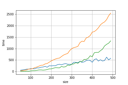
Fig. 6 Experimental runtime of 3 algorithms (orange, green, and blue curves).
In practice, the runtime curves are noisy, but we should be able to fit a curve that corresponds to the theoretical complexity on it. A simple trick to find if a curve corresponds to a given polynomial complexity \(\Theta(n^c)\) is to take the measured time \(t_1\) and \(t_2\) at sizes \(n\) and \(2n\) (for some arbitrary size value \(n\)), then we should have \(t_2/t_1 \approx 2^c\). So for a linear complexity, we should have a ratio \(t_2/t_1 \approx 2\), for a quadratic complexity, we should have a ratio \(t_2/t_1 \approx 4\), for a cubic complexity, we should have a ratio \(t_2/t_1 \approx 8\) and so on.
The measured ratio of algorithm 1 (green curve) is equal to , its runtime complexity is \(\Theta(n^3)\) is it coherent?
The measured ratio of algorithm 2 (blue curve) is equal to , its runtime complexity is \(\Theta(n^2)\) is it coherent?
The measured ratio of algorithm 3 (orange curve) is equal to , its runtime complexity is \(\Theta(n^2)\) is it coherent?
Programming exercise 1 : Implement selection sort and verify that the experimental runtime matches with the theoretical complexity in
the python notebook.
Programming exercise 2 : Implement insertion sort and verify that the experimental runtime matches with the theoretical complexity
in the python notebook.
We consider a sequence of algorithms alg_k parametrized by a positive integer k such that:
def alg_0(n):
  return n + 1
and for any integer k greater than 0:
def alg_k(n):
  res = n
  for i in range(n):
    res = alg_(k-1)(res) # note that the input of alg_(k-1) is the output of the previous call to alg_(k-1)
  return res
Give the runtime complexity of:
alg_0(n): Θ()
alg_1(n): Θ()
alg_2(n): Θ()
Those algorithms correspond to the fast-growing hierarchy, the complexity of alg_3 is already so large
that it can’t be expressed simply with classical mathematical notations.