Divide and Conquer

Divide and conquer is an algorithm design technic where a problem is recursively broken down into several smaller sub-problems until they become small enough so that simple solutions can be found. The solutions of the sub-problems are then recursively combined to find the solution to the original problem.

In this chapter, we will first recall some basic notions on recursion. Then we will study several examples of divide-and-conquer algorithms and we will see how to compute their runtime complexity. Finally, we will design and implement several divide-and-conquer algorithms.

Recursion

A function or an algorithm is said to be recursive if it calls itself. A recursive function implies to handle (at least) two cases:

• a base case: this is where we can compute and return the solution without having to make a recursive call

• a general case: where the problem is not simple enough to be solved directly and one or several recursive calls to simpler sub-problems are done.

Let’s look at a very simple example, the function that compute the factorial of an integer:

def factorial(n):
    if n <= 1:  # base case
        return 1  # end of the recursion
    else:  # general case
        factnm1 = factorial(n - 1)  #   recursive call to the simpler sub-problem (n is decreased by 1)
        return n * factnm1          #   return the solution deduced from the sub-problem solution

For example, calling factorial(4) will produce the following sequence of recursive function calls:

Fig. 15 At first, factorial(4) calls factorial(3), which calls factorial(2), which calls factorial(1). factorial(1) hits the base case and starts the second phase where we can unwind function calls by returning actual values. factorial(1) returns 1, which is used by factorial(2) to return its value 2 and so on.

It is of course crucial that the reduction into sub-problems always end on the base case after a finite number of recursive calls. Otherwise, the function is stuck in an infinite loop and in practice the program will crash with a stack overflow or a segmentation fault.

In more complicated cases, the algorithm contains several recursive calls to itself. Let’s consider the following example:

def algo(n):
    if n <= 1:  # base case
        return 1  # end of the recursion
    else:  # general case
        r1 = algo(n - 1)   # recursive call to the simpler sub-problem (n is decreased by 1)
        r2 = algo(n // 2)  # recursive call to the simpler sub-problem (n is divided by 2)
        return r1 + r2     # return solution deduced from the combination of the 2 sub-problem solutions

In this case, the sequence of recursive calls is more complex, it is called the call tree (see figure below). The length of the longest path in the call tree is called the recursion depth.

Fig. 16 The call tree generated by a call to algo(5). There is a total of 13 function calls. The longest path in the tree is denoted by red boxes: the recursion depth is thus equal to 5.

Note

A fundamental result of theoretical computer science is that any recursive function can be written as an iterative function (without recursion) and conversely. However, the iterative version of a recursive function is often more complex to write as a stack data structure must be used to emulate the call stack of functions (see your operating system course).

In order to understand the behavior of a recursive algorithm, it is important to be able to determine the recursion depth of the algorithm, i.e. in how many recursive calls do we reach the base case.

Consider the following recursive functions:

def rec1(n):
    if n <= 0:
        print("end")
    else:
        rec1(n - 1)

def rec2(n):
    if n <= 0:
        print("end")
    else:
        rec2(n - 2)

def rec3(n):
    if n <= 0:
        print("end")
    else:
        rec3(n // 2)

def rec4(n):
    if n <= 0:
        print("end")
    else:
        rec4(n // 3)

What is the recursion depth for the following function calls:

• rec1(3):

• rec1(6):

• rec2(3):

• rec2(6):

• rec3(4):

• rec3(16):

• rec4(4):

• rec4(16):

The recursive depth of these function growths like:

• rec1(n) = Ө()

• rec2(n) = Ө()

• rec3(n) = Ө()

• rec4(n) = Ө()

Consider the following recursive functions:

def ones1(n):
    if n == 0:
        print(1)
    else:
        ones1(n - 1)

def ones2(n):
    if n == 0:
        print(1)
    else:
        ones2(n - 1)
        ones2(n - 1)

def ones3(n):
    if n == 0:
        print(1)
    else:
        for i in range(1, n):
            ones3(n - 1)

def ones4(n):
    if n == 0:
        print(1)
    else:
        for i in range(1, 2**n):
            ones4(n - 1)

How many ones are printed by the call

• ones1(n):

• ones2(n):

• ones3(n):

• ones4(n):

Given a \(m\times n\) matrix of integers, give a \(O(m + n)\) time algorithm to check if a given integer \(x\) exists in the matrix. The matrix has the special property that each row is increasing, and each column is increasing.

Hint

Compare \(x\) to the last element \(y\) of the first row: what can you conclude if \(x\) is smaller than \(y\)? And if \(x\) is greater than \(y\)?

Binary search

Binary search is an algorithm to find the index of an element in a sorted array. Binary search leverages on the sorted nature of the array to split the search space in two at each step. The idea is the following one, at each step:

• if the array is empty: the element is not in the array, return -1

• otherwise: compare the value of the searched element with the element at the middle of the array:

  • if they are equal, the element is found, return the index of the middle element

  • if the searched element is smaller than the middle element, call binary search on the left sub-array

  • else call binary search on the right sub-array

Fig. 17 Binary search of the value 7 in the given sorted array. We start by comparing 7 to the element in the middle 14: as the array is sorted and as 7 is lower than 14, we know that 7 can only be on the left sub-array. The same reasoning is thus performed on the left sub-array: 7 is greater than 6; the searched element can thus only be somewhere between 6 and 14, and so on. (Image source *AlwaysAngry* on Wikipedia)

A possible pseudo-code for binary search is:

def binary_search(array, element, start=0, end=array.length):
    if start == end: # empty sub-array
        return -1;
    middle = (start + end) // 2
    if array[middle] == element:
        return middle;
    elif array[middle] > element:
        return binary_search(array, element, start, middle)
    else:
        return binary_search(array, element, middle + 1, end)

In the worst case, the element is not in the array, we have to do recursive calls until start equals end: the array is empty. At each call, we do:

• first, a constant (bounded) amount of work to handle the base case,

• and, if the array is not empty, a recursive call to the algorithm with an array size divided by 2.

Then, the worst-case runtime complexity \(T(n)\) (with \(n\) the length of the array), can be written:

\[\begin{split}T(n) = \begin{cases} c_0 & \textrm{ if } n=0 \\ c_1 + T(n/2) & \textrm{ otherwise,} \end{cases}\end{split}\]

with \(c_0\) and \(c_1\) two constants. We can then unwind the recursive equation:

\[\begin{split}\begin{align} T(n) & = c_1 + T(n/2) \\ & = c_1 + c_1 + T(n/4) \\ & = c_1 + c_1 + c_1 + T(n/8) \\ & = \ldots \\ & = i*c_1 + T(n/2^i), \end{align}\end{split}\]

and the recursion stops when:

\[\begin{split}\begin{align} n/2^i & = 1 \\ 2^i & = n \\ i & = \log_2(n) \end{align}\end{split}\]

Note that this is not completely rigorous as \(n\) and \(i\) are integers and the exact number of steps should be \(\lceil\log_2(n)\rceil + k\) with \(k\) a small integer that does not depend of \(n\). Hopefully, this does not affect the computation of the runtime complexity. The worst case complexity of binary search is thus:

\[\begin{split}\begin{align} T(n) & = i*c_1 + T(n/2^i) \\ & = \log_2(n)*c_1 + T(0) \\ & = \Theta(\log(n)) + c_0\\ & = \Theta(\log(n)) \end{align}\end{split}\]

Intuitively, this can be understood as: when dividing an array of size \(n\) by 2, it takes in the order of \(\log(n)\) steps to obtain an array of size 1. Moreover, as, at each step we perform a constant amount of work (without including the work done in the recursive calls), in the end we perform in the order of \(\log(n)\) times a constant amount of work and the total amount of work is also in the order of \(\log(n)\).

Binary search, taking advantage of the sorted nature of the array, thus achieves a better runtime complexity than the linear search algorithm viewed in the previous chapter.

As you may have noticed, in binary search, we only recurse on one side of the array. Therefore, there is no combine step and the binary search is a form of degenerate divide-and-conquer algorithm (it is sometime called decrease and conquer because of this). The following example will give a more complete view of the divide-and-conquer strategy

Consider an array \(a\) of numbers of size \(n\) such that all the elements are distinct. An element of the array is called a peak element if it is surrounded by smaller elements. Formally, the element at index \(i\) is a peak element if

• \(i=0\) and the array is of size 1, or

• \(i=0\) and \(a[i]>a[i+1]\), or

• \(i=n-1\) and \(a[i-1]<a[i]\), or

• \(0<i<n-1\) and \(a[i-1]<a[i]\) and \(a[i]>a[i+1]\)

For example, in the following array \([0, 2, 3, 1, 5, 4, 6]\), the peak elements are the values 3 (at index 2), 5 (at index 4), and 6 (at index 6).

1. Propose a linear time \(\Theta(n)\) algorithm in pseudo-code that returns the index of a peak element in an input array and -1 if there is no peak element (only possible if the input array is empty).

2. Adapt binary search to propose a logarithmic time \(\log(n)\) algorithm in pseudo-code that returns the index of a peak element in an input array and -1 if there is no peak element.

   Hint

   At a given position \(i\), if \(a[i]\) is not a peak element then either \(a[i-1] > a[i]\) and there is a peak element on the left of \(i\) or \(a[i] < a[i + 1]\) and there is a peak element ont he right of \(i\).

Merge sort

In the previous chapters, we have seen two sorting algorithms, insertion sort and selection sort, which both have a quadratic worst-case runtime. We will now see another sorting algorithm called merge sort based on the divide-and-conquer paradigm and which has a better runtime complexity.

Merge sort is based on the following observation: it is possible to merge two sorted arrays into a single sorted array in linear time.

Fig. 18 Merging two sorted arrays can be done in linear time with respect to the size of the two arrays.

The idea is simply to browse the two arrays in parallel. At each step, we select the smallest element among the current element of the first and the second arrays, we insert it at the back of the new merged array and we increase the current position by one in the selected array. Once we have exhausted all the elements of one of the input arrays, we just have to copy all the elements left in the other array in the result. Note that this procedure requires to allocate a new array.

We can then use this to design a recursive algorithm based on the following idea:

1. If the array has 0 or 1 element, it is already sorted: stop

2. Split the array in two

3. Sort each sub-array (recursive call)

4. Merge the two sub-arrays

Fig. 19 Principle of the merge sort.

The following figure shows a complete example.

Fig. 20 Sequence of calls for a merge sort on an array of size 8. The depth of the recursion is 4 (the last recursion step is trivial when arrays are of size 1) for a total of 15 calls to the merge sort algorithm (1 at depth 1, 2 at depth 2, 4 at depth 3, and 8 at depth 4).

Note that the amount of work done does not depend of the content of the input array: the best-case, worst-case and average-case runtime complexities are the same for merge sort. This runtime complexity \(T(n)\), with \(n\) the length of the array, can be written:

\[\begin{split}T(n) = \begin{cases} c_0 & \textrm{ if } n\leq 1 \\ c_1*n + 2*T(n/2) & \textrm{ otherwise.} \end{cases}\end{split}\]

with \(c_0\) and \(c_1\) two constants. We can then unwind the recursive equation:

\[\begin{split}\begin{align} T(n) & = c_1*n + 2*T(n/2) \\ & = c_1*n + 2*c_1*n/2 + 4*T(n/4) \\ & = c_1*n + c_1*n + 4*c_1*n/4 + 8*T(n/8) \\ & = \ldots \\ & = i*c_1*n + 2^i*T(n/2^i) \end{align}\end{split}\]

As with binary search, the size of the problem is divided by 2 at each step and the recursion stops in the order of \(\log_2(n)\) steps. This leads to:

\[\begin{split}\begin{align} T(n) & = i*c_1*n + 2^i*T(n/2^i) \\ & = \log_2(n) * c_1 * n + 2^{\log_2(n)}T(0) \\ & = \Theta(n\log(n)) + n*c_0\\ & = \Theta(n\log(n)) + \Theta(n) \\ & = \Theta(n\log(n)) \end{align}\end{split}\]

Compared to binary search, we also have in the order of \(\log(n)\) steps to perform. But, this time the amount of work to do at each step is not constant, it’s proportional to the size of the sub-problem. Moreover, the total size of the sub-problems at each step is indeed equal to the size of the whole problem (see for example Fig. 20: the total number of elements is the same at each line/step). Thus, we have \(\log(n)\) steps and at each step, the amount of work to do is in the order of \(n\), the total amount of work is thus in the order of \(\Theta(n\log(n))\)

The worst-case, best-case, and average-case runtime complexity of merge sort is thus \(\Theta(n\log(n))\) which is a significant improvement over the quadratic worst case runtime of selection sort and insertion sort. However, with the procedure given above, the merging of two sorted arrays requires to allocate a new array to store the result: the space complexity is thus in \(\Theta(n)\). In place versions of merge-sort exist, but they are rather complicated.

Implement merge sort and verify that the experimental runtime matches with the theoretical complexity.

Programming exercise : Implement merge sort and verify that the experimental runtime matches with the theoretical complexity in the python notebook

Note

We have seen that merge sort achieves a linearithmic runtime complexity for sorting an array. A fundamental question we can ask ourselves is: can we do better? It is in general very difficult to determine if a better algorithm (one with a better runtime complexity) exists for a given problem.

Unfortunatly, without further assumptions on the array to be sorted, the answer is no: in the worst case, a general sorting algorithm based on comparisons has to do in the order of \(n\log(n)\) operations. We can get an intuitive idea of this fundamental limit by taking an information theory point of view.

Sorting an array of \(n\) elements is equivalent to finding a permutation that sorts the elements of this array. A permutation is itself represented by an array of \(n\) integers containing the integers from 0 to \(n-1\) (for example a value of 4 at position 2 in the permutation array tells us that the element at position 2 in the original array should go at position 4 in the sorted array). Encoding a number in the range 0 to \(n-1\), requires \(\log_2(n)\) bits. As we have \(n\) numbers in the permutation array and each of this number requires \(\log_2(n)\) bits, there is a total of \(n\log_2(n)\) bits of information in the permutation array.

Assume that the input array contains \(n\) distinc numbers (all the numbers are distinct) with a completly random order. In this general case, there is a unique permutation that sorts this array and all the bits of the permutation array have to be determined. As the comparison between two numbers provides a single bit of information, any sorting algorithm has to perform at least in the order of \(n\log(n)\) comparisons to completely determine the permutation array that sorts the input array.

Note that, this does not prevent more efficient sorting algorithms to exist if we do stronger hypothesis on the content of the input array. For example, if the number of unique values in the array is small compared to its size (for example we have an array of 1 million elements storing numbers between 0 and 255), then, intuitively, many different permutation arrays will sort the same input array and linear time complexity sorting algorithm exist in this case.

Assume that we can merge three sorted arrays of size \(n\) in linear time \(\Theta(n)\). What is the worst-case runtime complexity of a merge sort that split the input array in 3 instead of 2, with \(n\) the size of the input? Θ()

Optional question: Propose an algorithm in pseudo-code that performs the merge of 3 sorted arrays in linear time.

You are given \(k\) sorted arrays \(A_1, \ldots, A_k\), each containing \(n\) elements. The goal is to merge these \(k\) sorted arrays into one sorted array with \(kn\) elements.

1. Consider the algorithm that first merges \(A_1\) with \(A_2\), then merges this result with \(A_3\), then merges this result with \(A_4\) and so on. What is the runtime complexity of this algorithm: Θ()

2. Propose an algorithm based on divide and conquer whose running time is \(O (nk\log(k))\). In the complexity analysis, you can consider that the variable of the recurence equation is \(k\) and \(n\) is a non constant factor (you cannot remove it from the complexity analysis).

Assume that we have an array \(a\) of numbers of size \(n\). The sub-array ranging from index \(i\) (included) to index \(j>i\) (excluded) is denoted by \(a[i:j]\). The sum of the elements \(\sum a[i:j]\) of a sub-array \(a[i:j]\) is simply the sum of all the elements in the sub-array: \(\sum a[i:j] = \sum_{k=i}^{k<j} a[k]\). The goal of the problem is to find the maximum sub-array (the starting and the end indices): the sub-array of maximum sum. By convention the maximum sub-array of an empty array is the empty array and its sum is equal to \(-\infty\).

Example: assume that \(a=[5, -8, 7, -4, 3, 3, -9, 8, -2, 1 ]\)

• the sum of the sub-array \(a[1:4]\) is equal to -5

• the sum of the sub-array \(a[2:8]\) is equal to 8

• the maximum sub-array sub-array is \(a[2:6]\), its sum is 9

All the algorithms bellow should return 3 values: the first index of the sub-array, the last index of the sub-array (exclusive) and the sum of the sub-array.

1. Propose a quadratic runtime \(\Theta(n^2)\) algorithm based on a brute force approach (compute the sum of all the sub-arrays and keep the maximum).

2. Propose a linear runtime \(\Theta(n)\) algorithm for finding the maximum sub-array that contains a given index \(k\) (i.e. a sub-array \(\sum a[i::j]\) such that \(i\leq k < j\)). Hint: consider all left of k sub-arrays in the form \(a[i::k]\) and all right of k sub-arrays in the form \(a[k::j]\).

3. Propose a divide-and-conquer algorithm with a linearithmic runtime \(n\log(n)\) to find the maximum sub-array. Hint: question 2 should be useful for the combine step.

Quick sort

Quick sort is another sorting algorithm based on the divide-and-conquer paradigm. Contrarily to merge sort which has a trivial divide step (just split the array in half) and a non trivial combine step (merge two sorted arrays), quick sort relies on a non trivial divide step and a trivial combine one.

In quick sort, the input array is partitioned in two by picking an element, called the pivot, and then moving all the elements smaller than the pivot on the left side of the array and all the others on the right side. We have thus divided the input array in two parts such that all the elements of the left part are smaller than the ones of the right part. It is then sufficient to (recursively) sort each side of the array.

1. If the array has 0 or 1 element, it is already sorted: stop

2. Select a pivot element

3. Reorder the array elements such that all elements with a value lower (resp. greater) than the pivot are on the left (resp. on the right) of the pivot.

4. Sort sub-array on the left of the pivot and the sub-array on the right of the pivot (recursive calls)

The following figure shows an example of execution of quicksort.

Fig. 21 Sequence of calls for a quick sort on an array of size 7. Here the pivot (in red) is always chosen as the first element in the array. The whole algorithm is done in place (no new array is created). We can see that the array are generally not split evenly, which implies that the depth is not the same in all the execution branches.

The reoder step of quick sort can be done in linear time and inplace (without allocating a new array). A possible algorithm to do this proceeds as follows:

1. Select the pivot as the last element of the array

2. Browse the array from the first element to the last element - 1 and accumulate the elements smaller than the pivot at the beginning of the array

3. Move the pivot to the correct position (after all the elements smaller than the pivot)

A possible implementation is:

def reorder_array(array):

    pivot = array[-1]  # pivot is the last element of the array
    i = -1  # Temporary pivot index

    # Browse the array and move the elements smaller than the pivot to the left of the array
    for j in range(len(array) - 1):
        if array[j] <= pivot:  # If the current element is less than or equal to the pivot
            i += 1  # Move the temporary pivot index forward
            array[i], array[j] = array[j], array[i]  # Swap the current element with the element at the temporary pivot index

    # Move the pivot element to the correct pivot position
    i += 1
    array[i], array[-1] = array[-1], array[i]
    return i  # the pivot index

Exercise: applies this algorithm to the following arrays

• [8, 1, 3] : the reordered array is [] the final index of the pivot is

• [1, 2, 3, 4] : the reordered array is [] the final index of the pivot is

• [4, 3, 2, 1] : the reordered array is [] the final index of the pivot is

• [8, 3, 2, 1, 5, 6, 4] : the reordered array is [] the final index of the pivot is

Programming exercise : Implement reorder_array in the python notebook Note that the function in the notebook takes two extra parameters: the start and the end index of the sub-array to reorder.

Note that after reordering the elements of the array, the pivot is indeed correctly sorted: if the pivot ends at the index \(k\) this means that the pivot is the \(k+1\)-th smallest element of the array.

The runtime complexity analysis of quick sort is more difficult than the one of merge sort as the two sub-arrays in the recursive calls generally do not have the same size. Moreover the position of the split indeed depends of a non specified par of the algorithm: the pivot selection.

In the following, we consider the reordering algorithm presented in the previous exercise where the pivot is the last element of the array.

Worst case

If the array is already sorted, then this pivot selection will always create a division where the first sub-array contains \(n-1\) elements and the second sub-array is empty.

Fig. 22 Example of worst case execution of quick sort when the pivot is the first element of the array.

In this case, the runtime complexity \(T(n)\) (with \(n\) the length of the array), can be written:

\[\begin{split}T(n) = \begin{cases} c_0 & \textrm{ if } n\leq 1 \\ c_1*n + T(n-1) & \textrm{ otherwise.} \end{cases}\end{split}\]

with \(c_0\) and \(c_1\) two constants. We can unwind the recursive equation:

\[\begin{split}\begin{align} T(n) & = c_1*n + T(n-1) \\ & = c_1*n + c_1*(n-1) + T(n-2) \\ & = c_1*n + c_1*(n-1) + c_1*(n-2) + T(n-3) \\ & = \ldots \\ & = c_1*(1 + 2 + \ldots + n)\\ & = c_1*(n(n+1)/2)\\ & = \Theta(n^2) \end{align}\end{split}\]

The worst case is thus quadratic \(\Theta(n^2)\), which is worse than the one of merge sort.

Best case

In the best case, the pivot will always split the array in two equal parts (with at most a size difference of 1). This brings us back to the case of the merge sort and the best-case runtime complexity is thus in \(\Theta(n\log(n))\).

Average case

If we consider all possible permutations of the input array with equal probability, then we can show that the average runtime complexity of quick sort is in \(\Theta(n\log(n))\). The formal proof of this result is a bit cumbersome but we can get an intuition of why this result holds thanks to the following observation.

Assume that, in any case, the choice of the pivot enables to split the array such that the length of the smallest sub-array is greater than a fixed percentage \(c\) of the length of the array. For example if \(c=0.02\), this means that after the split of an array of size \(n\), the length of the smallest sub-array is at least \(0.02n\) (and thus the length of the other sub-array is at most \(0.98n\)). In the ideal case \(c=0.5\), the array is split evenly.

Then, the longest branch in the call tree, is composed of the calls where the array size if divided by at least a factor \(1/(1-c)\): the recursion depth is thus equal to \(\log_{1/(1-c)}(n)= \Theta(\log(n))\). As the amount of work done at each step of the recursion is still bounded by \(O(n)\), the total amount of work is bounded by \(O(n\log(n))\).

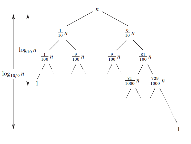
Fig. 23 Example of a quick sort call tree with a pivot selection ensuring \(c=1/10\). The shortest path in the tree is on the left and has a length equal to \(\log_{10}(n)\). The longest path is on the right and has a depth equal to \(\log_{10/9}(n)\). Up to the depth \(\log_{10}(n)\), the amount of work per level is in the order of \(\Theta(n)\). In the level belows, the amount of work per level is less but still bounded by \(O(n)\). In this end, the total amount of work is thus bounded by \(O(n\log(n))\). (Source: Introduction to Algorithms by Thomas H. Cormen, Charles E. Leiserson, Ronald L. Rivest and Clifford Stein)

So, we see that the splits can be unbalanced by an arbitrarily large constant factor and the runtime is still linearithmic. In practice, with a randomly distributed array, an arbitrary pivot selection method (for example chose the first element), will lead to uniformly random splits: in other words, very bad splits are far less probable than not too bad ones. So even if the worst-case cannot be excluded, it is extremely unlikely to happen and the average case has indeed the same runtime complexity as the best case.

Programming exercise : Implement quick sort and verify that the experimental runtime matches with the theoretical complexity in the python notebook

What happens if you try to sort an already sorted array of size 10000? Explain.

A selection algorithm is an algorithm for finding the \(k\)-th smallest number in an array of size \(n\). When \(k=n/2\), this element is called the median.

1. Propose a selection algorithm with a linearithmic runtime complexity \(\Theta(n\log(n))\) (you can use a sorting algorithm).

2. Propose a selection algorithm with a variation of quick-sort: this algorithm is called quick-select. Recall that after a reordering step in quick-sort, the pivot is indeed put at its correct position in the sorted array.

3. Show that this algorithm has a quadractic worst case runtime complexity \(O(n^2)\).

4. Argue that in average, the runtime complexity of quick-select is \(O(n)\).

   Hint

   Assume that the choice of the pivot always enables to split the array such that the length of the largest sub-array is at most equal to \(c*n\) with \(c\) a constant strictly smaller than 1. Write the recurence equation and remember that \(\lim_{n\rightarrow\infty}\sum_{i=0}^{n} a^i\) is always bounded when \(0\leq a < 1\).

Going further: Strassen’s Matrix multiplication

Matrix multiplication is a common problem in engineering and data science where it often involves very large matrices. It is thus of prime importance to have efficient algorithms to perform such operation. Formally, given two square matrices \(A\) and \(B\) of size \(n \times n\), the result of the multiplication \(M=AB\) of \(A\) and \(B\) is a square matrix of the same size defined by the line-column product formula:

\[m_{i,j} = \sum_{k=1}^{n}a_{i,k}b_{k,j}\]

Propose a naive algorithm to compute the product of two square matrices of size \(n \times n\).

The complexity of this algorithm is: Θ()

Let’s see how we can apply a divide-and-conquer strategy to the matrix multiplication problem. In all previous problems, we were processing a 1d array that was split in two sub-arrays. Here, as we are working with square matrices, we will partition each matrix into 4 square sub-matrices:

\[\begin{split}A = \begin{bmatrix} A_{11} & A_{12} \\ A_{21} & A_{22}\end{bmatrix}, \quad B = \begin{bmatrix} B_{11} & B_{12} \\ B_{21} & B_{22}\end{bmatrix}, \quad M = \begin{bmatrix} M_{11} & M_{12} \\ M_{21} & M_{22}\end{bmatrix}\end{split}\]

Beware that in these equations \(A_{11}, B_{11}, M_{11}, A_{12}, \ldots\) are matrices, not numbers! We then have:

\[\begin{split}\begin{align} M_{11} & = A_{11}B_{11} + A_{12}B_{21} \\ M_{12} & = A_{11}B_{12} + A_{12}B_{22} \\ M_{21} & = A_{21}B_{11} + A_{22}B_{21} \\ M_{22} & = A_{21}B_{12} + A_{22}B_{22} \end{align}\end{split}\]

For example, let,

\[\begin{split}A = \begin{bmatrix} 1 & 2 & 3 & 4 \\ 5 & 6 & 7 & 8 \\ 9 & 10 & 11 & 12 \\ 13 & 14 & 15 & 16\end{bmatrix}, \quad B = \begin{bmatrix} 21 & 22 & 23 & 24 \\ 25 & 26 & 27 & 28 \\ 29 & 30 & 31 & 32 \\ 33 & 34 & 35 & 36\end{bmatrix}\end{split}\]

We have:

\[\begin{split}\begin{align} M_{11} & = A_{11}B_{11} + A_{12}B_{21} \\ & = \begin{bmatrix} 1 & 2 \\ 5 & 6\end{bmatrix}\begin{bmatrix} 21 & 22 \\ 25 & 26\end{bmatrix} + \begin{bmatrix} 3 & 4 \\ 7 & 8\end{bmatrix}\begin{bmatrix} 29 & 30 \\ 33 & 34\end{bmatrix}\\ & = \begin{bmatrix} 1 * 21 + 2 * 25 & 1*22+2*26 \\ 5*21+6*25 & 5*22+6*26\end{bmatrix} + \begin{bmatrix} 3*29+4*33 & 3*30+4*34 \\ 7*29+8*33 & 7*30+8*34\end{bmatrix}\\ & = \begin{bmatrix} 1 * 21 + 2 * 25 + 3*29+4*33& 1*22+2*26+3*30+4*34 \\ 5*21+6*25+7*29+8*33 & 5*22+6*26+7*30+8*34\end{bmatrix} \end{align}\end{split}\]

We recover the classical definition of matrix multiplication.

Now let’s study the time complexity of this algorithm. Let \(T(n)\) be the number of operations used to process 2 matrices of size \(n\times n\). We have:

\[\begin{split}T(n) = \begin{cases} c_0 \textrm{ if } n=1 \\ c_1n^2 + 8T(n/2) \textrm{ otherwise.}\end{cases}\end{split}\]

with \(c_0\) and \(c_1\) two constants. The base case happens when \(n=1\): which is indeed just the multiplication of two scalar numbers. In the general case, we need to compute the 4 sub-matrices. Each sub-matrix requires 2 matrix multiplications (recursive calls) and 1 matrix addition (\(n^2\) scalar additions).

Let’s unwind the equation:

\[\begin{split}\begin{align} T(n) & = c_1*n^2 + 8T(n/2) \\ & = c_1*n^2 + 8*c_1\left(\frac{n}{2}\right)^2+ 8^2T(n/4)\\ & = c_1*n^2 + 2*c_1*n^2 + 8^2*c_1\left(\frac{n}{4}\right)^2 8^3T(n/8)\\ & = c_1*n^2(1+ 2 + 4 + \ldots + 2^i) + 8^iT(N/2^i)\\ & = c_1*n^2(2^{i+1} - 1) + 8^iT(N/2^i) \end{align}\end{split}\]

The recursion stops after \(i=\log_2(n)\) steps, which gives:

\[\begin{split}\begin{align} T(n) & = c_1*n^2(2*2^{\log_2(n)} - 1) + 8^{\log_2(n)}T(0) \\ & = c_1*n^2(2n+1) + 8^{\log(n)/\log(2)}c_0 \\ & = \Theta(n^3) + 8^{\log_8(n)*\log(8)/\log(2)}c_0\\ & = \Theta(n^3) + (8^{\log_8(n)})^{\log(8)/\log(2)}c_0\\ & = \Theta(n^3) + n^{\log_2(8)}c_0\\ & = \Theta(n^3) + n^{3}c_0\\ & = \Theta(n^3) \end{align}\end{split}\]

So we have introduced quite a lot of complexity and we didn’t improve the time complexity. The problem is that our transformation with sub-matrices did not reduce the number of operations: we have just reorganized the order in which operations are done. This can be fixed with the following rewriting of the equations. The Strassen algorithm defines the new matrices:

\[\begin{split}\begin{align} C_1 & = (A_{11} + A_{22})(B_{11} + B_{22}) \\ C_2 & = (A_{21} + A_{22})B_{11} \\ C_3 & = A_{11}(B_{12}-B_{22})\\ C_4 & = A_{22}(B_{21}-B_{11})\\ C_5 & = (A_{11} + A_{12})B_{22}\\ C_6 & = (A_{21} - A_{11})(B_{11} + B_{12})\\ C_7 & = (A_{12} - A_{22})(B_{21} + B_{22}) \end{align}\end{split}\]

We now have:

\[\begin{split}\begin{align} M_{11} & = C_1 + C_4 - C_5 + C_7 \\ M_{12} & = C_3 + C_5 \\ M_{21} & = C_2 + C_4 \\ M_{22} & = C_1 - C_2 + C_3 + C_6 \end{align}\end{split}\]

The interesting thing here is that, there is only 7 matrix multiplications in the definition of the matrices \(C_1, \ldots, C_7\) instead of 8 needed in the previous definition: we need to do 1 less recursive call!

The new recurrence equation for the time complexity is:

\[\begin{split}T(n) = \begin{cases} c_0 \textrm{ if } n=1 \\ c_1n^2 + 7T(n/2) \textrm{ otherwise.}\end{cases}\end{split}\]

with \(c_0\) and \(c_1\) two constants. Let’s unwind the equation:

\[\begin{split}\begin{align} T(n) & = c_1*n^2 + 7T(n/2) \\ & = c_1*n^2 + 7*c_1\left(\frac{n}{2}\right)^2+ 7^2T(n/4)\\ & = c_1*n^2 + (7/4)*c_1*n^2 + 7^2*c_1\left(\frac{n}{4}\right)^2 7^3T(n/8)\\ & = c_1*n^2(1+ 7/4 + (7/4)^2 + \ldots + (7/4)^i) + 7^iT(N/2^i)\\ & = c_1*n^2\frac{(7/4)^i-1}{7/4-1} + 7^iT(N/2^i) \end{align}\end{split}\]

The recursion stops after \(i=\log_2(n)\) steps, which gives:

\[\begin{split}\begin{align} T(n) & = c_1*n^2\frac{(7/4)^{\log_2(n)}-1}{7/4-1} + 7^{\log_2(n)}T(N/2^i) \\ & = c_1*n^2\frac{((7/4)^{\log_{7/4}(n)})^{\log(7/4)/\log(2)}-1}{7/4-1} + n^{\log(7)/\log(2)}c_0\\ & = c_1*n^2\frac{n^{\log_2(7/4)}-1}{7/4-1} + n^{\log_2(7)}c_0\\ & = \Theta(n^{2 + \log_2(7/4)}) + \Theta(n^{\log_2(7)})\\ & = \Theta(n^{2 + \log_2(7) - log_2(4)}) + \Theta(n^{\log_2(7)})\\ & = \Theta(n^{\log_2(7)}) + \Theta(n^{\log_2(7)}) \\ & = \Theta(n^{\log_2(7)}) \\ & \approx \Theta(n^{2.807}) \end{align}\end{split}\]

which is a significant improvement over the \(\Theta(n^{3})\) naïve algorithm.

Write the pseudo-code for Strassen’s matrix multiplication algorithm assuming that the size of the input matrices is a power of 2.

Programming exercise : Implement Strassen matrix multiplication in the python notebook