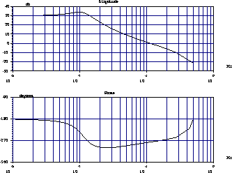
Figure 5: Bode plot of the Model
The first think we notice with the result of the identification process is :

Figure 5: Bode plot of the Model
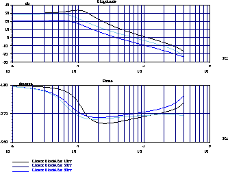
This conclusions seems to be available for the all the subject of the same class (e.g. the healthy one). For example the gap in term of frequencies responses between healthy subject is very short and the gain decreasing take place in any case for the same game of frequencies (less than a decade centered on 0.01Hz). Another interesting conclusion we can give just looking on the frequencies responses of the different linear models is the following. The upper bound frequencie of the filter is decreasing with the volumen of the balloon. We can see this purpose on the next figure (6). We wont discuss the consequence of this effect in the next section.

Figure 6: Bode plot of 3 models for the same subject
Currently the model we obtain as (in transfer function form) this kind of values
Where the sampling interval is 0.2 second.
We will try now to look on a continuous linear model in order to find a
mechanical device usable for our prothesis project. To establish all the frequencies responses
curves, we work first with Matri ![]() . But all the graphs of this paper are made with
. But all the graphs of this paper are made with ![]() lab
the freeware of the META2 group from INRIA.
lab
the freeware of the META2 group from INRIA.