Evaluation#
Evaluation is the process of assessing the performance of a model on a dataset not used during training. This process can be performed at the end of training or periodically during training to monitor the model’s performance. During evaluation, gradients are not computed, and the model is set to evaluation mode to disable features like dropout and batch normalization updates. Below are the typical steps for evaluation.
Disable gradient computation.
Set the model to evaluation mode.
Iterate through the dataset with a DataLoader.
Perform a forward pass to compute predictions.
Compare predictions to ground truth using metrics such as accuracy, precision, recall, etc.
For a more detailed explanation of this topic, you can refer to this tutorial.
Note
A custom evaluation loop is defined in the training.py script. Download this file to your working directory to reproduce the examples presented in these tutorials.
Metrics in PyTorch#
While PyTorch provides a robust framework for building and training models, it does not include built-in support for evaluation metrics like accuracy, precision, recall, etc. Fortunately, third-party libraries have been developed to provide ready-to-use metrics, such as Scikit-Learn, TorchMetrics, and TorchEval.
TorchEval#
TorchEval is a library developed by the PyTorch team that provides a variety of evaluation metrics for classification, regression, and other common tasks. It is designed to have two interfaces for each metric: a functional API that computes the metric in a single call, and a class-based API that maintains state across multiple calls. The class-based API is of particular interest for evaluation loops, as it allows us to create metric objects with three important methods.
reset(): Reset the metric to its initial state, preparing it for a new evaluation run.update(): Update the metric with new data (e.g., predictions and targets). This method is called for each mini-batch during evaluation.compute(): Compute the metric value by aggregating the data accumulated from previousupdate()calls. This method is called at the end of an evaluation run.
Note
If you followed the instructions to set up your environment, you already have torcheval installed.
Evaluation loop#
The main purpose of the evaluation loop is to assess the model’s performance on a validation or test dataset. The evaluation loop is similar to the training loop, but with some important differences.
Evaluation mode → Layers like dropout and batch normalization are not updated.
No backpropagation → Gradients are not computed, model parameters remain unchanged.
Metrics instead of loss → Task-specific metrics are evaluated instead of loss function.
The following code snippet implements a minimal evaluation loop using TorchEval for metrics computation. Notice the usage of torch.inference_mode() decorator to disable gradient computation.
Show code cell source
import torch
from torch.utils.data import DataLoader
from torcheval.metrics import Metric


@torch.inference_mode()
def evaluation_loop(model: torch.nn.Module,
                    loader: DataLoader,
                    metrics: dict[str, Metric]) -> dict:

    # Device transfer
    device = torch.device("cuda" if torch.cuda.is_available() else "cpu")
    model.to(device)

    # Metric reset
    for metric in metrics.values():
        metric.reset()
        metric.to(device)

    # Evaluation mode
    model.eval()

    # Data iteration
    for inputs, labels in loader:

        # Forward pass
        inputs = inputs.to(device)
        labels = labels.to(device)
        outputs = model(inputs)

        # Metric update
        for metric in metrics.values():
            metric.update(outputs, labels)

    # Metric computation
    results = {name: metric.compute() for name, metric in metrics.items()}

    return results
The Trainer class defined in the training.py script includes a simple evaluation loop that is enough for most use cases. If you need more control over the evaluation process, you can implement a custom evaluation loop starting from the evaluation_loop function defined above.
Example#
Let’s demonstrate how to use the Trainer class by training a simple network on the MNIST dataset and running evaluations at different stages of the training process. We start by importing the required libraries.
import torch
from torch import nn, optim
from torch.utils.data import DataLoader
from torcheval.metrics import MulticlassAccuracy, MulticlassConfusionMatrix
from torchvision.datasets import MNIST
from torchvision.transforms import v2
import matplotlib.pyplot as plt
from training import Trainer
First, we load the MNIST dataset with a minimal preprocessing pipeline that converts the images to tensors. We also create two DataLoader to iterate over the training and test datasets in mini-batches.
preprocess = v2.Compose([v2.ToImage(), v2.ToDtype(torch.float32, scale=True)])

train_ds = MNIST('.data', train=True,  download=True, transform=preprocess)
test_ds  = MNIST('.data', train=False, download=True, transform=preprocess)

train_loader = DataLoader(train_ds, batch_size=64, shuffle=True)
test_loader  = DataLoader(test_ds,  batch_size=256, shuffle=False)
Then, we define the model, loss function, and optimizer.
model = nn.Sequential(
    nn.Flatten(),
    nn.Linear(28*28, 128),
    nn.ReLU(),
    nn.Linear(128, 10)
)

optimizer = optim.Adam(model.parameters(), lr=1e-3)

loss_fn = nn.CrossEntropyLoss()
Next, we create a Trainer object and register the metrics we want to monitor during training. In this case, we use multiclass accuracy as our metric.
trainer = Trainer()

trainer.set_metrics(accuracy=MulticlassAccuracy())
Finally, we train the model for a few epochs, using the test DataLoader for evaluation after each epoch.
epochs  = 5
history = trainer.fit(model, train_loader, loss_fn, optimizer, epochs, test_loader)
===== Training on mps device =====
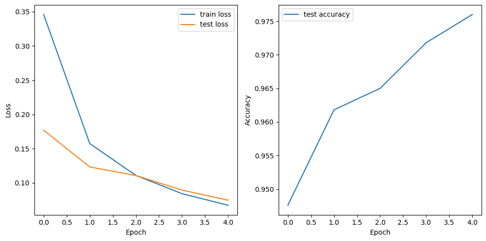
Epoch  1/5: 100%|██████████| 938/938 [00:38<00:00, 24.45it/s, accuracy=0.9476, train_loss=0.3461, valid_loss=0.1770]
Epoch  2/5: 100%|██████████| 938/938 [00:37<00:00, 25.29it/s, accuracy=0.9618, train_loss=0.1573, valid_loss=0.1232]
Epoch  3/5: 100%|██████████| 938/938 [00:36<00:00, 25.36it/s, accuracy=0.9650, train_loss=0.1108, valid_loss=0.1106]
Epoch  4/5: 100%|██████████| 938/938 [00:36<00:00, 25.37it/s, accuracy=0.9718, train_loss=0.0842, valid_loss=0.0894]
Epoch  5/5: 100%|██████████| 938/938 [00:36<00:00, 25.78it/s, accuracy=0.9760, train_loss=0.0672, valid_loss=0.0746]
The loss function and all the validation metrics are recorded during training and returned in a dictionary. We can plot the training loss and the validation metrics to visualize the model performance over time.
Show code cell source
plt.figure(figsize=(10, 5), tight_layout=True)
plt.subplot(1, 2, 1)
plt.plot(history['train_loss'], label='train loss')
plt.plot(history['valid_loss'], label='test loss')
plt.xlabel('Epoch')
plt.ylabel('Loss')
plt.legend()
plt.subplot(1, 2, 2)
plt.plot(history['accuracy'], label='test accuracy')
plt.xlabel('Epoch')
plt.ylabel('Accuracy')
plt.legend()
plt.show()
We can also evaluate the trained model on the test set by calling the eval method of the Trainer, which returns a dictionary of metric values.
results = trainer.eval(model, test_loader)

print(f"Test accuracy: {results['accuracy']:.2%}")
Test accuracy: 97.60%
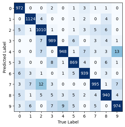
To evaluate the model on a different metric or dataset, we can reuse the existing Trainer object. We just need to set the new metrics and call the .eval() method with the test DataLoader.
trainer.set_metrics(confmat=MulticlassConfusionMatrix(10))

results = trainer.eval(model, test_loader)
Show code cell source
confmat = results['confmat'].int()
num_classes = confmat.shape[0]

plt.imshow(confmat, cmap='Blues', norm=plt.Normalize(0, 30))
plt.xlabel('True Label')
plt.ylabel('Predicted Label')
plt.xticks(range(num_classes))
plt.yticks(range(num_classes))
for i in range(num_classes):
    for j in range(num_classes):
        plt.text(j, i, confmat[i, j].item(), ha='center', va='center', color='white' if i == j else 'black')