
Deep Metric Learning#
Many machine-learning problems go beyond standard classification. An image-retrieval system, for instance, must rank a gallery according to its relevance to a query; a verification system must determine whether two samples correspond to the same identity; a clustering system must group related examples without relying on predefined output labels.
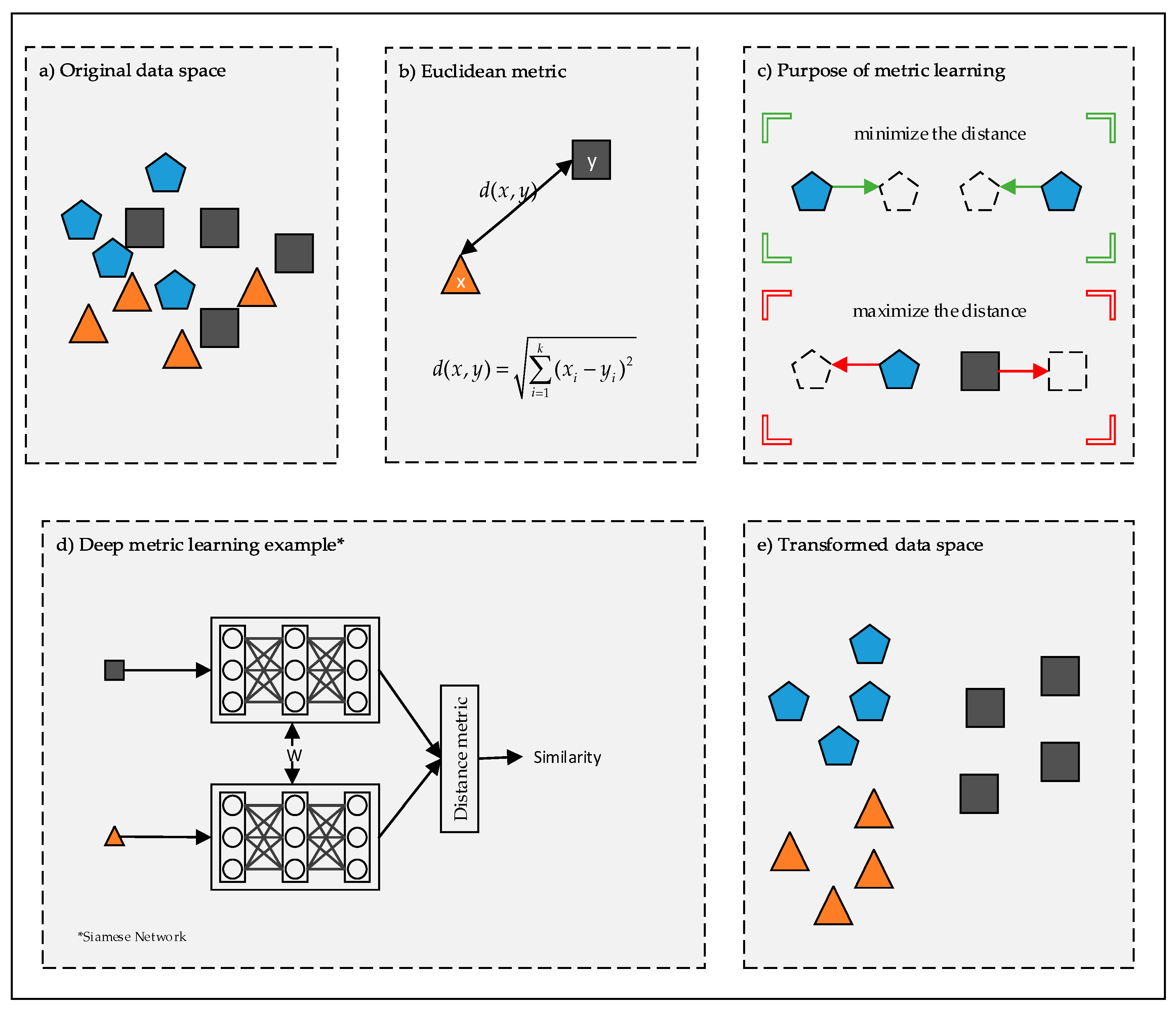
Deep metric learning addresses these problems by training a neural network \(f_\theta\) that maps an input to a finite-dimensional vector known as an embedding. Training encourages related examples to receive similar embeddings and unrelated examples to receive dissimilar embeddings. Similarity is quantified through a distance function \(\mathcal{D}\) defined in the embedding space. Given a pair of examples \((x_i, x_j)\) and a label \(s_{ij}\) indicating whether they are related, the training objective is to ensure the following.
The meaning of “similarity” is entirely task-dependent. It may indicate that two images show the same digit, the same person, the same product, or objects judged visually similar by human annotators. Metric learning therefore does not discover a universal notion of similarity; it learns the notion encoded in the training data.
Representation learning#
A classifier maps an input to one of the classes represented during training. Its final output layer is therefore tied to a particular label set. Instead, an embedding model produces a reusable representation that can support several downstream operations, including retrieval, verification, clustering, and nearest-neighbor classification. This distinction is especially important when the system must handle classes that were not observed during training. For example, a face-embedding model may be trained on one set of identities but later used to compare entirely new individuals. Good performance on unseen classes is an intended property of the embedding, but it is not guaranteed. It must be measured using validation and test data whose classes are appropriately separated from those used for training.
Metric learning also differs from classical dimensionality-reduction methods such as principal component analysis (PCA) and t-SNE. These methods typically transform features that have already been constructed. Deep metric learning instead learns the feature extractor and the embedding jointly, using an objective that directly reflects the desired similarity relationships. In addition, t-SNE is primarily intended for low-dimensional visualization. Its plots may reveal qualitative structure, but they do not replace quantitative evaluation of retrieval or verification performance.
Distance and similarity functions#
Embeddings can be compared using several functions. Common choices include the following.
Euclidean distance: \(\mathcal{D}(z_i,z_j) = \| z_i-z_j \|_2\).
Cosine similarity: \(\cos(z_i,z_j) = \dfrac{z_i^\top z_j}{\|z_i\|_2 \, \|z_j\|_2}\).
Dot product: \(z_i^\top z_j\).
These measures treat vector magnitude differently. Euclidean distance depends on both the directions and the norms of the embeddings. The dot product also increases with vector magnitude, whereas cosine similarity depends only on the angle between vectors. A common modeling choice is therefore to apply L2 normalization, where \(\epsilon>0\) prevents division by zero.
The normalized embeddings lie on the unit hypersphere. For unit vectors, cosine similarity and the dot product are identical. Their Euclidean distance is also determined entirely by their angle, since \(\|\hat{z}_i-\hat{z}_j\|_2^2 = 2 - 2\hat{z}_i^\top \hat{z}_j\). Thus, maximizing cosine similarity is equivalent to minimizing Euclidean distance between normalized embeddings. Moreover, the distance between any two normalized embeddings is always bounded between 0 and 2, due to the triangle inequality.
This bounded scale makes margins and decision thresholds easier to interpret and tune. Normalization is nevertheless a modeling decision, not a universal requirement. In some tasks, the embedding norm may carry useful information that should not be removed.
Metric learning objectives#
Metric-learning objectives differ mainly in which examples they compare simultaneously and how they express the desired geometry.
Pair-based objectives operate on pairs of examples. Positive pairs are encouraged to become close, while negative pairs are encouraged to remain separated. Contrastive loss is the standard example. These objectives express similarity directly, but their effectiveness depends strongly on how informative pairs are selected. Many randomly sampled pairs may already satisfy the objective and therefore contribute little to learning.
Triplet objectives compare three examples: an anchor, a positive example related to the anchor, and a negative example unrelated to the anchor. Rather than requiring an absolute distance, the objective requires the positive to be closer to the anchor than the negative, usually by a specified margin. Triplet objectives naturally encode ranking, but their performance depends on selecting useful triplets. Triplets that are already correctly ordered provide little training signal, whereas excessively difficult or mislabeled triplets may destabilize optimization.
Multi-sample objectives compare each embedding with many candidates at once. NT-Xent and InfoNCE-style losses are prominent examples. For a given anchor, a positive example is contrasted against several negatives, often using all other suitable examples in the minibatch. Because many relationships contribute to each update, these objectives can use a minibatch more efficiently than independently sampled pair or triplet losses. Their behavior, however, depends on batch composition, temperature scaling, and the number and quality of available negatives.
Proxy-based objectives represent classes using learned vectors called proxies. Instead of comparing an embedding with many individual examples, the loss compares it with one or more learned class representatives. Proxy-NCA is an example of this approach.
Classification-based objectives, such as ArcFace and CosFace, modify the geometry of a classification problem by introducing angular margins. Although they are trained using class labels, their purpose is to produce embeddings with strong separation and compact within-class structure.
The boundaries between these families are not strict. Many modern objectives combine pairwise, ranking, multi-sample, and classification-based ideas.
Evaluation#
The evaluation protocol must reflect the intended use of the embedding model. For example, if the model will be used to retrieve similar examples from a gallery, then retrieval metrics are appropriate. If it will be used to verify whether two examples match, then verification metrics are appropriate. In either case, the evaluation should be performed on held-out data whose classes were not observed during training.
Retrieval#
Retrieval evaluation uses two collections:
a query set, containing the examples for which results are requested;
a gallery, containing the candidate examples to be ranked.
For each query, the gallery is sorted by increasing distance or decreasing similarity. Recall@K measures whether at least one relevant gallery item appears among the first \(K\) retrieved results. It is useful when finding a single correct match is sufficient. Precision@K measures the fraction of the first \(K\) retrieved items that are relevant. It is useful when multiple correct matches are expected.
When the query and gallery are drawn from the same collection, the query example itself must be excluded from its ranking. Otherwise, its distance to itself is zero, producing an artificially optimistic result.
Verification#
Verification determines whether two examples should be considered a match. Given a distance threshold \(\tau\), the decision rule is that a pair \((z_i,z_j)\) is considered a match if their distance is less than or equal to \(\tau\). The threshold is part of the model-selection procedure, and must therefore be chosen using validation data. Test data should be evaluated only after the threshold and all other hyperparameters have been fixed.
Verification performance can be summarized using metrics such as accuracy, ROC curves, or true-positive rate at a specified false-positive rate. The appropriate metric depends on the costs associated with false acceptances and false rejections.
Representation Collapse#
A metric-learning model is useful only if its embeddings preserve meaningful distinctions between inputs. A degenerate solution occurs when every input is mapped to approximately the same vector. This phenomenon is called representation collapse. A collapsed embedding may make positive pairs close, but it cannot distinguish unrelated examples and therefore cannot support meaningful ranking or verification.
Negative pairs, ranking margins, and the denominators of contrastive objectives help prevent collapse by requiring different examples to remain distinguishable. Collapse can be diagnosed by inspecting quantities such as embedding variance, pairwise distances, cosine-similarity distributions, and retrieval performance. Visual inspection may complement these diagnostics, but a visually structured two-dimensional projection does not by itself demonstrate that the original embedding space is useful.
Chapter Overview#
In this chapter, we develop and implement three metric-learning approaches:
balanced contrastive loss for pair-based supervision;
robust online mining for triplet-based learning;
pair-supervised retrieval using an NT-Xent objective.
These methods illustrate how the choice of training objective, sample construction, embedding geometry, and evaluation protocol jointly determines the quality of a learned metric space.