Feature Extraction#
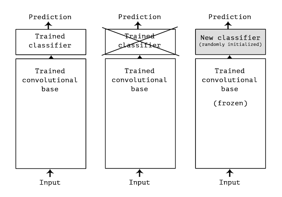
Convolutional networks used for image classification consist of two main components: a convolutional backbone, composed of convolution and pooling layers, followed by a classification head made up of fully-connected layers. Broadly speaking, the convolutional backbone extracts generic features from the input image, while the classification head interprets these features to make a prediction. Transfer learning takes advantage of this architecture to repurpose the convolutional backbone of a pre-trained network. Instead of training an entire model from scratch, the pre-trained backbone is reused to extract features from new data. Then, a new classifier is trained on top of these extracted features. This particular approach is commonly referred to as feature extraction.
In this tutorial, we will explain how to use feature extraction on the cats-vs-dogs dataset. We will download a pre-trained model from the TorchVision library, get the convolutional backbone from the model, and use it to extract features from images of cats and dogs. We will then train a new classifier on top of these features.
Analysis of MobileNetV3#
Let’s take a look at a model that has been pre-trained on the ImageNet dataset. There are plenty of models to choose from in the TorchVision library. In this tutorial, we use MobileNetV3 for its speed and efficiency.
from torchvision.models import mobilenet_v3_large, MobileNet_V3_Large_Weights

weights = MobileNet_V3_Large_Weights.DEFAULT

pretrained = mobilenet_v3_large(weights=weights)
We inspect MobileNetV3 architecture using the TorchInfo library, which provides a detailed summary of the model’s layers, output shapes, number of parameters, and more.
Note
If you followed the instructions to set up your environment, you already have torchinfo installed.
To have a breakdown of the output shapes, we need to specify the expected input size of the model. MobileNetV3 expects images of size 224x224 with three color channels (RGB). The batch size is set to 1 for simplicity. We also set the depth parameter to limit the level of detail in the summary.
Show code cell source
from torchinfo import summary

summary(pretrained, input_size=(1, 3, 224, 224), depth=1, col_width=16, col_names=["input_size", "output_size"], row_settings=["var_names"])
============================================================================================
Layer (type (var_name))                                      Input Shape      Output Shape
============================================================================================
MobileNetV3 (MobileNetV3)                                    [1, 3, 224, 224] [1, 1000]
├─Sequential (features)                                      [1, 3, 224, 224] [1, 960, 7, 7]
├─AdaptiveAvgPool2d (avgpool)                                [1, 960, 7, 7]   [1, 960, 1, 1]
├─Sequential (classifier)                                    [1, 960]         [1, 1000]
============================================================================================
Total params: 5,483,032
Trainable params: 5,483,032
Non-trainable params: 0
Total mult-adds (Units.MEGABYTES): 216.62
============================================================================================
Input size (MB): 0.60
Forward/backward pass size (MB): 70.46
Params size (MB): 21.93
Estimated Total Size (MB): 92.99
============================================================================================
As indicated above, MobileNetV3 consists of three modules.
features- A series of convolutional and pooling layers that extract the input image into feature maps.avgpool- A layer that averages the channels of the feature maps (3D) to produce a feature vector (1D).classifier- A series of fully-connected layers that predicts the class logits from the feature vector.
Classification head#
Let’s visualize the classification head of MobileNetV3. The summary shows that the first layer expects a vector of size 960, while the last layer produces a vector of size 1000. We take note of the input size because we will need this information to build a new classifier on top of the extracted features.
Show code cell source
summary(pretrained.classifier, input_size=(1, 960), col_names=["input_size", "output_size"])
==========================================================================================
Layer (type:depth-idx)                   Input Shape               Output Shape
==========================================================================================
Sequential                               [1, 960]                  [1, 1000]
├─Linear: 1-1                            [1, 960]                  [1, 1280]
├─Hardswish: 1-2                         [1, 1280]                 [1, 1280]
├─Dropout: 1-3                           [1, 1280]                 [1, 1280]
├─Linear: 1-4                            [1, 1280]                 [1, 1000]
==========================================================================================
Total params: 2,511,080
Trainable params: 2,511,080
Non-trainable params: 0
Total mult-adds (Units.MEGABYTES): 2.51
==========================================================================================
Input size (MB): 0.00
Forward/backward pass size (MB): 0.02
Params size (MB): 10.04
Estimated Total Size (MB): 10.07
==========================================================================================
Convolutional backbone#
Let’s visualize the convolutional backbone of MobileNetV3. We notice that the expected input has 3 channels, while the produced output has 960 channels. This aligns with the classification head.
Show code cell source
summary(pretrained.features, input_size=(1, 3, 224, 224), depth=1, col_names=["input_size", "output_size"])
===============================================================================================
Layer (type:depth-idx)                        Input Shape               Output Shape
===============================================================================================
Sequential                                    [1, 3, 224, 224]          [1, 960, 7, 7]
├─Conv2dNormActivation: 1-1                   [1, 3, 224, 224]          [1, 16, 112, 112]
├─InvertedResidual: 1-2                       [1, 16, 112, 112]         [1, 16, 112, 112]
├─InvertedResidual: 1-3                       [1, 16, 112, 112]         [1, 24, 56, 56]
├─InvertedResidual: 1-4                       [1, 24, 56, 56]           [1, 24, 56, 56]
├─InvertedResidual: 1-5                       [1, 24, 56, 56]           [1, 40, 28, 28]
├─InvertedResidual: 1-6                       [1, 40, 28, 28]           [1, 40, 28, 28]
├─InvertedResidual: 1-7                       [1, 40, 28, 28]           [1, 40, 28, 28]
├─InvertedResidual: 1-8                       [1, 40, 28, 28]           [1, 80, 14, 14]
├─InvertedResidual: 1-9                       [1, 80, 14, 14]           [1, 80, 14, 14]
├─InvertedResidual: 1-10                      [1, 80, 14, 14]           [1, 80, 14, 14]
├─InvertedResidual: 1-11                      [1, 80, 14, 14]           [1, 80, 14, 14]
├─InvertedResidual: 1-12                      [1, 80, 14, 14]           [1, 112, 14, 14]
├─InvertedResidual: 1-13                      [1, 112, 14, 14]          [1, 112, 14, 14]
├─InvertedResidual: 1-14                      [1, 112, 14, 14]          [1, 160, 7, 7]
├─InvertedResidual: 1-15                      [1, 160, 7, 7]            [1, 160, 7, 7]
├─InvertedResidual: 1-16                      [1, 160, 7, 7]            [1, 160, 7, 7]
├─Conv2dNormActivation: 1-17                  [1, 160, 7, 7]            [1, 960, 7, 7]
===============================================================================================
Total params: 2,971,952
Trainable params: 2,971,952
Non-trainable params: 0
Total mult-adds (Units.MEGABYTES): 214.11
===============================================================================================
Input size (MB): 0.60
Forward/backward pass size (MB): 70.44
Params size (MB): 11.89
Estimated Total Size (MB): 82.93
===============================================================================================
To retrieve the exact size of the output, we can pass a random tensor of shape (…, 3, 224, 224) through the backbone. We then inspect the shape of the resulting tensor.
import torch

batch = torch.randn(1, 3, 224, 224)

with torch.inference_mode():
    output = pretrained.features(batch)

print('Feature shape:', tuple(output.shape[1:]))
Feature shape: (960, 7, 7)
Standalone feature extractor#
There are two ways to implement feature extraction.
Standalone approach. Run the convolutional backbone over the whole dataset, store its output in a PyTorch Tensor, and then use this data as input to a standalone classifier. This solution is very fast and cheap to run, because it only requires running the pre-trained backbone once for every input image, which is by far the most expensive part of the pipeline. However, this technique would not allow us to leverage data augmentation at all.
End-to-end approach. Create a new model that combines the pre-trained backbone (with frozen weights) and a new classification head (with trainable weights). This allows us to use data augmentation, because every input image is going through the convolutional backbone every time it is seen by the model. However, fthis technique is far more expensive than the first one.
We will cover the standalone approach in this tutorial.
Show code cell source
import torch
import torch.nn.functional as F
from torch import nn, optim
from torch.utils import data
from torchvision.datasets import ImageFolder
from sklearn.model_selection import train_test_split
import matplotlib.pyplot as plt
Dataset with preprocessing#
We start by loading the cats-vs-dogs dataset and dividing it into training and test sets. We assume that the data has been downloaded and extracted to the .data/cats-vs-dogs/PetImages directory.
# TODO: Change this to the path where the dataset is stored
data_path = '.data/cats_vs_dogs/PetImages'

# MobileNetV3 preprocessing
weights = MobileNet_V3_Large_Weights.DEFAULT
preprocess = weights.transforms()

# Function that converts labels to float tensors
torch_float = lambda x: torch.tensor(x, dtype=torch.float)

# Setup the dataset with preprocessing
dataset = ImageFolder(data_path, transform=preprocess, target_transform=torch_float)

# Split the indices
train_idx, test_idx = train_test_split(range(len(dataset)), stratify=dataset.targets, test_size=0.2, shuffle=True, random_state=42)

# Create the subsets
train_ds = data.Subset(dataset, train_idx)
test_ds  = data.Subset(dataset, test_idx)
See also
The tutorial Dataset from files explains how to download the cats-vs-dogs dataset.
Extracting features#
Let’s extract features from the cats-vs-dogs dataset by running the convolutional backbone over the whole dataset. We will create a function extract_features that takes a model and a dataset as input, and returns a TensorDataset with the extracted features and the corresponding labels.
Show code cell source
from tqdm import tqdm

def extract_features(model: nn.Module,
                     dataset: data.Dataset,
                     batch_size: int=64) -> data.TensorDataset:

    prev_device = next(model.parameters()).device
    device = torch.device('cuda' if torch.cuda.is_available() else 'mps' if torch.mps.is_available() else 'cpu')

    model = model.to(device).eval()

    dataloader = data.DataLoader(dataset, batch_size=batch_size, shuffle=False)

    features = []
    labels = []

    for images, target in tqdm(dataloader, desc='Extracting features'):
        with torch.inference_mode():
            images = images.to(device)
            feats = model(images)
            features.append(feats.cpu())
            labels.append(target)

    features = torch.cat(features)
    labels = torch.cat(labels)

    model = model.to(prev_device)

    return data.TensorDataset(features, labels)
WARNING: The code below may take some time to run (about 15 minutes on CPU).
pretrained = mobilenet_v3_large(weights=weights)

pretrained.eval()  # Evaluation mode for feature extraction

extracted_train_ds = extract_features(pretrained.features, train_ds)
extracted_test_ds  = extract_features(pretrained.features, test_ds)
Extracting features: 100%|██████████| 293/293 [02:49<00:00,  1.73it/s]
Extracting features: 100%|██████████| 74/74 [00:43<00:00,  1.71it/s]
Let’s print the size of the extracted features. We expect the size to be 960x7x7.
Show code cell source
print('Extracted features (train):', tuple(extracted_train_ds.tensors[0].shape))
print('Extracted features (test):  ', tuple(extracted_test_ds.tensors[0].shape))
Extracted features (train): (18728, 960, 7, 7)
Extracted features (test):   (4682, 960, 7, 7)
Defining a new classifier#
Now that we have the extracted features, we can train a new classifier on top of them. We will use a simple feedforward neural network with two hidden layers. The input size of the network should match the size of the extracted features, while the output size is a single value representing the logit for the positive class.
class Classifier(nn.Module):

    def __init__(self):
        super().__init__()
        input_dim = 960 * 7 * 7
        self.fc = nn.Linear(input_dim, 256)
        self.dropout = nn.Dropout(0.5)
        self.out = nn.Linear(256, 1)

    def forward(self, x):
        x = torch.flatten(x, 1)
        x = self.fc(x)
        x = torch.relu(x)
        x = self.dropout(x)
        x = self.out(x)
        return torch.squeeze(x, -1)
Note
The model output is squeezed so that it has shape (batch_size,) instead of (batch_size, 1). At the same time, labels are converted to float tensors during preprocessing. Together, these steps prevent shape and type mismatch errors when using BCEWithLogitsLoss as a loss function.
Training the classifier#
Let’s import Trainer from the training.py file and BinaryAccuracy from TorchEval.
from training import Trainer
from torcheval.metrics import BinaryAccuracy
Training is very fast, since we only have to deal with two fully-connected layers.
train_loader = data.DataLoader(extracted_train_ds, batch_size=64, shuffle=True)
test_loader  = data.DataLoader(extracted_test_ds, batch_size=128)

loss_fn = nn.BCEWithLogitsLoss()

model = Classifier()
optimizer = optim.Adam(model.parameters(), lr=0.001, amsgrad=True)
epochs = 5

trainer = Trainer()
trainer.set_metrics(accuracy=BinaryAccuracy())

history = trainer.fit(model, train_loader, loss_fn, optimizer, epochs, test_loader)
===== Training on mps device =====
Epoch  1/5: 100%|██████████| 293/293 [00:21<00:00, 13.37it/s, accuracy=0.9850, train_loss=0.0760, valid_loss=0.0414]
Epoch  2/5: 100%|██████████| 293/293 [00:12<00:00, 23.94it/s, accuracy=0.9883, train_loss=0.0224, valid_loss=0.0428]
Epoch  3/5: 100%|██████████| 293/293 [00:12<00:00, 24.03it/s, accuracy=0.9891, train_loss=0.0101, valid_loss=0.0471]
Epoch  4/5: 100%|██████████| 293/293 [00:12<00:00, 22.87it/s, accuracy=0.9887, train_loss=0.0061, valid_loss=0.0624]
Epoch  5/5: 100%|██████████| 293/293 [00:12<00:00, 22.90it/s, accuracy=0.9889, train_loss=0.0048, valid_loss=0.0603]
Let’s plot the loss of the model computed on the training and test sets.
Show code cell source
plt.figure(figsize=(10, 5), tight_layout=True)
plt.subplot(1, 2, 1)
plt.plot(history['train_loss'], label='Train loss')
plt.plot(history['valid_loss'], label = 'Test loss')
plt.xlabel('Epoch')
plt.ylabel('Loss')
plt.legend()
plt.subplot(1, 2, 2)
plt.plot(history['accuracy'], label='test accuracy')
plt.xlabel('Epoch')
plt.ylabel('Accuracy')
plt.legend()
plt.show()
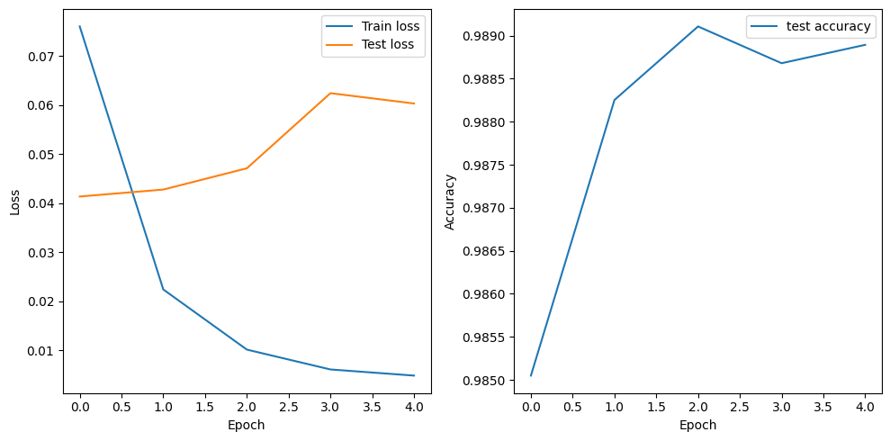
The plots indicate that we are overfitting almost from the start, despite using dropout with a fairly large rate. Data augmentation may help to prevent overfitting in this case, but we need to use the end-to-end approach to leverage it (not covered in this tutorial).
Evaluation#
Finally, we evaluate the model on the test set and print the classification accuracy.
Show code cell source
ans = trainer.eval(model, test_loader)

print(f"Test accuracy: {ans['accuracy']:.2%}")
Test accuracy: 98.89%
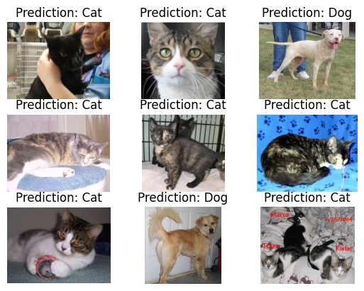
Let’s also plot some images from the test set and their corresponding predictions.
Show code cell source
# Device of the classifier
device = next(model.parameters()).device

# Images without preprocessing
raw_data = ImageFolder(data_path)

# Random image indices
n = 9
idx = torch.randint(0, len(raw_data), (n,))

# Retrieve original images
images, labels = zip(*[raw_data[i] for i in idx])

with torch.inference_mode():

    # Extract features
    batch = torch.stack([preprocess(img) for img in images])
    features = pretrained.features(batch)

    # Predict
    features = features.to(device)
    outputs = model(features)

# Plot
for i in range(n):
    plt.subplot(n//3, 3, i+1)
    plt.imshow(images[i])
    plt.title(f'Prediction: {"Dog" if outputs[i] > 0 else "Cat"}')
    plt.axis('off')
plt.show()
Summary#
In this tutorial, we learned how to use feature extraction to repurpose a pre-trained convolutional backbone for a new classification task. We downloaded a pre-trained MobileNetV3 from the TorchVision library, extracted features from the cats-vs-dogs dataset, and trained a new classifier on top of these features. The classifier achieved an impressive accuracy of 99% on the test set, which is not surprising given the simplicity of the dataset and its similarity to the ImageNet dataset.
Here are some key takeaways from this tutorial.
Why don’t we reuse the pre-trained classification head? Because the representations learned by the classifier will necessarily be very specific to the set of classes that the model was trained on.
Should we always reuse the entire convolutional backbone? The level of generality (and therefore reusability) of the representations extracted by specific convolution layers depends on the depth of the layer in the model. Layers that come earlier in the model extract local, highly generic feature maps (such as visual edges, colors, and textures), while layers higher-up extract more abstract concepts (such as “cat ear” or “dog eye”). So if your new dataset differs a lot from the dataset that the original model was trained on, you may be better off using only the first few layers of the model to do feature extraction, rather than using the entire convolutional backbone.