Training a Neural Network#
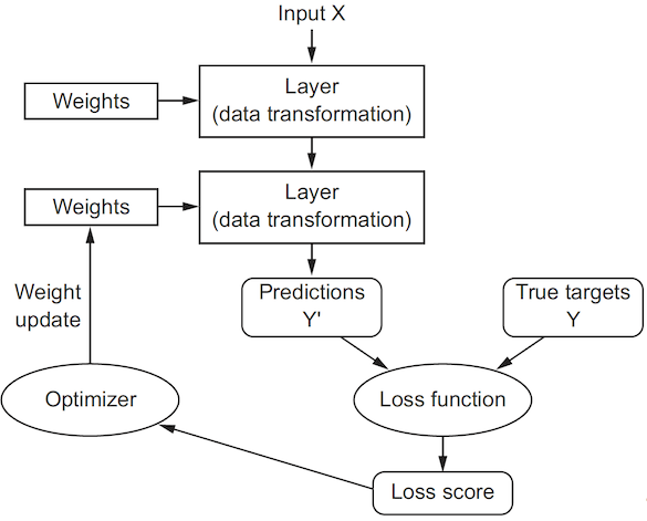
Initially, right after the neural network is created, the parameters of all layers are filled with small random values. This step is called random initialization. At this point, the network merely implements a series of random transformations. The next step is to gradually adjust these parameters based on the available data. This process is called training and consists of repeating the following steps as long as necessary.
Data sampling: A batch of data (inputs and targets) are randomly selected from the training set.
Forward pass: The inputs are passed through the network, and the outputs are computed.
Loss computation: The mismatch between the network outputs and the targets is measured.
Backward pass: The gradients of the loss with respect to the network parameters are computed.
Parameters update: The network parameters are updated using the computed gradients.
Eventually, the network learns to make accurate predictions on the training data by minimizing the loss function. In this tutorial, we will explain how to implement the training process using PyTorch.
Preparation#
Building a deep learning pipeline always starts with the decision of the task to solve and the dataset to use. In this tutorial, we will focus on a standard image classification task using the MNIST dataset of handwritten digits. The dataset consists of 60,000 training images and 10,000 test images of size 28x28 pixels. Each image contains a handwritten digit from 0 to 9, and the goal is to classify the images into one of the digits.
Show code cell source
import torch
from torch import nn, optim
from torch.utils.data import DataLoader
import torch.nn.functional as F
import torchvision.transforms.v2 as v2
from torchvision.datasets import MNIST
import matplotlib.pyplot as plt
Dataset#
We load the MNIST dataset with a preprocessing pipeline that converts the images into PyTorch tensors and normalizes them to have values between 0 and 1.
preprocess = v2.Compose([v2.ToImage(), v2.ToDtype(torch.float32, scale=True)])

train_ds = MNIST('.data', train=True,  download=True, transform=preprocess)
test_ds  = MNIST('.data', train=False, download=True, transform=preprocess)
Neural network#
For classifying the MNIST digits, we define a simple feedforward neural network that flattens the inputs and passes them through two fully-connected layers. The first layer has 512 neurons and a ReLU activation. The second layer has no activation since we will use the cross-entropy loss, which includes a softmax activation. The number of input in the first layer and the number of outputs in the last layer are specified as arguments to the constructor.
class SimpleNet(nn.Module):

    def __init__(self, input_dim, num_classes):
        super().__init__()
        self.flatten = nn.Flatten()
        self.linear1 = nn.Linear(input_dim, 512)
        self.linear2 = nn.Linear(512, num_classes)

    def forward(self, x):
        y = self.flatten(x)
        y = self.linear1(y)
        y = F.relu(y)
        y = self.linear2(y)
        return y
Loss function#
To control the output of a neural network, we need to be able to measure how far this output is from what we expected. This is the job of the loss function. It takes the prediction of the network and the expected target (what you wanted the network to output), and computes a distance score, capturing how well the network has done on this specific sample. The loss function is a key component of the training process, as it guides the optimization algorithm to adjust the network’s parameters in the right direction.
PyTorch provides a list of predefined loss functions. Choosing the right loss function for the right problem is extremely important, as a network will take any shortcut it can to minimize the loss. Fortunately, when it comes to common problems such as classification and regression, there are simple guidelines we can follow to choose the correct loss function.
Binary cross-entropy for a two-class classification.
Categorical cross-entropy for a many-class classification problem.
Mean squared error for a regression problem.
Handwritten digit classification is a many-class classification problem, so we will use the categorical cross-entropy loss function. This is called nn.CrossEntropyLoss in PyTorch.
loss_fn = nn.CrossEntropyLoss()
Note
You don’t need to include a softmax activation in the network when using nn.CrossEntropyLoss, as this function computes the softmax and the cross-entropy loss together. Conversely, if you are using nn.LogSoftmax as the output activation, then you should use nn.NLLLoss instead.
Optimizer#
The central idea behind deep learning is to adjust the parameters of a neural network using the gradient of the loss function. This is possible because the gradient is basically a vector that tells us in which direction we should move each parameter to reduce the loss. The optimizer is the algorithm responsible for adjusting the network’s parameters based on the computed gradients. The most common optimizer is stochastic gradient descent (SGD), but there are many different optimizers available in PyTorch, such as ADAM and RMSProp, that work better for different kinds of models and data.
To construct an Optimizer, we have to give it an iterable containing the parameters to optimize. In this case, we provide it with all the network parameters, which can be iterated over using the parameters() method. We can also specify optimizer-specific options, such as the learning rate.
model = SimpleNet(28*28, 10)

optimizer = optim.Adam(model.parameters(), lr=1e-3)
Note
The parameters to optimize must be tensors that have their requires_grad attribute set to True. All trainable parameters in a PyTorch model have this attribute set by default.
Training loop#
At this point, we have all the pieces to start training our neural network. But here comes the tricky part: how do we put all these pieces together? PyTorch does not answer this question for us, since it is designed as a low-level library that provides the building blocks for deep learning, but does not impose any specific way to use them. Over the years, several third-party libraries have been developed to provide high-level APIs for training neural networks, such as PyTorch Lightning. These libraries can save time and reduce boilerplate. However, it is instructive to understand how training works under the hood.
Note
A custom training loop is defined in the training.py script. Download this file to your working directory to reproduce the examples presented in these pages.
Implementation#
A good way to structure a training loop is to separate the per-batch logic from the boilerplate code that drives the loop itself. Conceptually, we can break down the implementation into two functions.
train_step(): This function will update the network’s parameters on a single batch of data.Trainer: This class will manage the overall training process. It provides a.fit()method that iterates over the dataset in batches and callstrain_step()to perform the actual training work for each batch.
We will now look at a minimal implementation of these two components.
The code snippet below shows the function that trains the model on a single batch of data. The assumption is that the batch is a tuple containing the inputs and the targets, the model takes the inputs as its only argument, and the loss function takes the model outputs and the targets as its arguments.
def train_step(model: nn.Module,
               batch: tuple[torch.Tensor, torch.Tensor],
               loss_fn: nn.Module,
               optimizer: optim.Optimizer,
               device: torch.device):

    # Data transfer
    inputs, labels = batch
    inputs = inputs.to(device)
    labels = labels.to(device)

    # Forward pass
    outputs = model(inputs)

    # Backward pass
    loss = loss_fn(outputs, labels)
    loss.backward()

    # Model update
    optimizer.step()
    optimizer.zero_grad()
The next code snippet shows the class that manages the training process. Notice that the fit() method delegates the processing of each batch to the function defined above. This separation allows for greater flexibility, as the training loop can be reused by replacing only the train_step() function.
class Trainer:

    def fit(self,
            model: nn.Module,
            loader: DataLoader,
            loss_fn: nn.Module,
            optimizer: optim.Optimizer,
            epochs: int):

        # Device transfer
        device = torch.device("cuda" if torch.cuda.is_available() else "cpu")
        model.to(device)

        # Training mode
        model.train()

        # Data iteration
        for epoch in range(epochs):
            for batch in loader:
                train_step(model, batch, loss_fn, optimizer, device)
While this code is functional and can be used to train a neural network, it lacks many features that are useful in practice, such as validation, logging, and checkpointing. You are advised to use a more complete implementation, such as the one provided in the training.py script or a third-party library.
Usage example#
Let’s demonstrate how to use the Trainer class. We start by importing it from the training.py file.
from training import Trainer
Next, we will train the model for 10 epochs, using a batch size of 512 and a learning rate of \(10^{-3}\). Note that these hyperparameters are passed directly to the data loader and the optimizer, respectively.
model = SimpleNet(28*28, 10)

loader = DataLoader(train_ds, batch_size=512, shuffle=True)
loss_fn = nn.CrossEntropyLoss()
optimizer = optim.Adam(model.parameters(), lr=1e-3)

trainer = Trainer()
history = trainer.fit(model, loader, loss_fn, optimizer, epochs=10)
===== Training on mps device =====
Epoch  1/10: 100%|██████████| 118/118 [00:17<00:00,  6.93it/s, train_loss=0.5068]
Epoch  2/10: 100%|██████████| 118/118 [00:15<00:00,  7.67it/s, train_loss=0.2141]
Epoch  3/10: 100%|██████████| 118/118 [00:15<00:00,  7.68it/s, train_loss=0.1551]
Epoch  4/10: 100%|██████████| 118/118 [00:15<00:00,  7.72it/s, train_loss=0.1185]
Epoch  5/10: 100%|██████████| 118/118 [00:15<00:00,  7.69it/s, train_loss=0.0967]
Epoch  6/10: 100%|██████████| 118/118 [00:15<00:00,  7.64it/s, train_loss=0.0796]
Epoch  7/10: 100%|██████████| 118/118 [00:15<00:00,  7.65it/s, train_loss=0.0653]
Epoch  8/10: 100%|██████████| 118/118 [00:15<00:00,  7.76it/s, train_loss=0.0560]
Epoch  9/10: 100%|██████████| 118/118 [00:15<00:00,  7.68it/s, train_loss=0.0471]
Epoch 10/10: 100%|██████████| 118/118 [00:15<00:00,  7.52it/s, train_loss=0.0421]
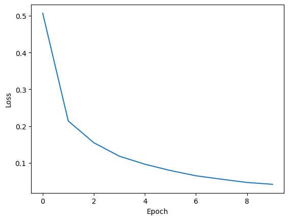
The fit() method tracks the average loss computed over each epoch, which is also returned as a list in a dictionary. This information is useful to visualize the training process and ensure that the model is learning. We expect the training loss to decrease over time, indicating that the model is improving its performance on the training data. If the loss is not decreasing, it may be a sign that the learning rate is too high, or that the model architecture is not suitable for the problem.
Show code cell source
plt.plot(history['train_loss'])
plt.xlabel('Epoch')
plt.ylabel('Loss')
plt.show()
Inference#
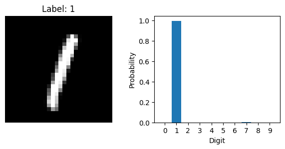
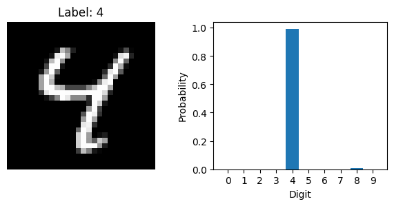
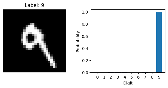
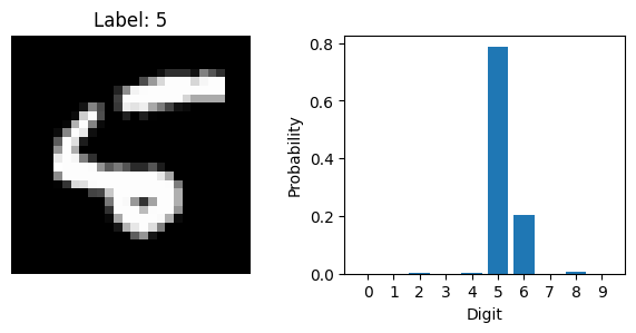
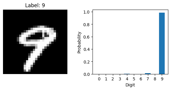
Now that the model is trained, we can use it to make predictions on new data. Let’s select a few images from the test set and ask the model to predict the digit in each one. We will also plot the images to see what the model is working with.
Show code cell source
# Get the device of the model
device = next(model.parameters()).device

for i in range(5, 10):

    # Get a sample
    image, label = test_ds[i]

    # Move image to device
    image = image.to(device)

    # Make prediction
    with torch.inference_mode():
        image = image.unsqueeze(0)
        scores = model(image)
        probs = F.softmax(scores, dim=1)

    # Visualize
    plt.figure(figsize=(6, 3), tight_layout=True)
    plt.subplot(1, 2, 1)
    plt.imshow(image.squeeze().cpu(), cmap='gray')
    plt.title(f'Label: {label}')
    plt.axis('off')
    plt.subplot(1, 2, 2)
    plt.bar(range(10), probs.squeeze().cpu())
    plt.xticks(range(10))
    plt.xlabel('Digit')
    plt.ylabel('Probability')
    plt.show()
Summary#
In this tutorial, we learned how to train a neural network using PyTorch. Specifically, we discussed how to choose a loss function, select an optimizer, and implement the training loop. We also learned how to make predictions with the trained model. Next, we will discuss how to evaluate the trained model.