Network Architecture#
Let’s take a practical look at a very simple convolutional network (CNN) for MNIST digit classification, a task that you have already been through using a fully-connected network.
Show code cell source
import torch
import torch.nn.functional as F
import torchvision.transforms.v2 as v2
from torchvision.datasets import MNIST
Image data#
The whole point of using a convolutional network is to be able to use images as input. But what is an image? It is a grid of pixels, where each pixel has a value representing the color intensity at that point. In the case of a grayscale image, the pixel value is a single number between 0 and 255. In the case of a color image, the pixel value is a 3-tuple of numbers between 0 and 255, each representing the intensity of one of the three color channels: red, green, and blue.
PyTorch represents images as 3D Tensors. The first dimension is the number of color channels, the second dimension is the height of the image, and the third dimension is the width of the image. So a grayscale image of size 28x28 pixels is represented as a tensor of shape (1, 28, 28), whereas a color image of the same size is represented as a tensor of shape (3, 28, 28).
Image Size = (channels, height, width)
This is the default representation used by PyTorch, which is called the channel-first format. However, it is also possible to use the channel-last format, where the channel dimension comes after the height and width dimensions. A PyTorch blog explains that the channel-last format performs better and is considered best practice. The reason is because XNNPACK (the kernel acceleration library used by PyTorch) expects all inputs to be in channel-last format.
This won’t make too much of a difference when working with small datasets and simple models. But keep it in mind for when you’re working on larger image datasets and more complex convolutional neural networks.
MNIST dataset#
As usual, we load the MNIST dataset with a preprocessing pipeline that converts the images into PyTorch tensors and normalizes them to have values between 0 and 1. We covered this topic in a previous tutorial, so we won’t go into too much detail here.
preprocess = v2.Compose([v2.ToImage(), v2.ToDtype(torch.float32, scale=True)])

train_ds = MNIST('.data', train=True,  download=True, transform=preprocess)
test_ds  = MNIST('.data', train=False, download=True, transform=preprocess)
Let’s take a look at the first image in the training set to confirm that the channel-first format is being used.
image, label = train_ds[0]

print('Image Size:', *image.shape)
Image Size: 1 28 28
Note
By default, PyTorch uses the channel-first format for images.
Creating LeNet-5#
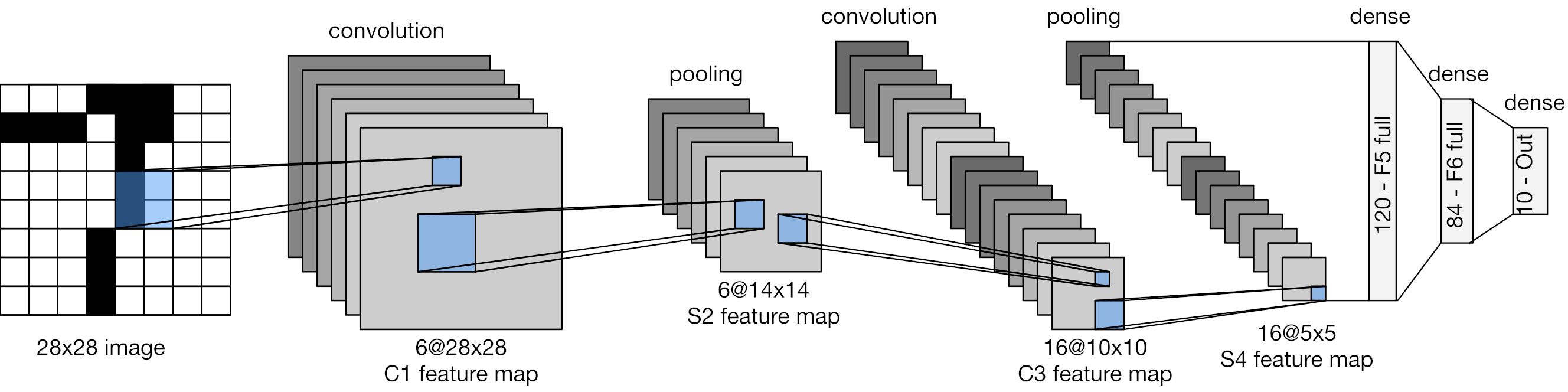
The LeNet-5 architecture was proposed by Yann LeCun in 1998. It was one of the first convolutional neural networks and was designed to classify handwritten digits. The architecture consists of two convolutional layers alternating with max-pooling layers, then a flattening layer followed by three fully-connected layers. The input to the network is a grayscale image of size 28x28 pixels, whereas the output is a vector of size 10, representing the scores for each of the 10 classes. Let’s implement this architecture in PyTorch.
Convolutional backbone#
A ConvNet always starts off with convolutional and pooling layers. In our case, we stack two convolutional layers, alternated with pooling layers.
Convolutional layers require us to specify the number of input channels and the number of output channels. The latter corresponds to the number of trainable filters that will be convolved with the input. We also need to specify the size of each filter, which is 5x5 in LeNet-5. We use a padding of 2 in the first layer, so that the spatial dimensions of the input tensor will remain the same after the convolution.
Pooling layers require us to specify the spatial dimensions of the pooling window, and optionally the strides, which defaults to the same value as the pooling window. In this case, we use a 2x2 window, which means that the spatial dimensions of the input tensor will be halved after the pooling operation.
class Backbone(torch.nn.Module):

    def __init__(self):
        super().__init__()
        self.conv1 = torch.nn.Conv2d(1,  6, kernel_size=5, padding=2)
        self.conv2 = torch.nn.Conv2d(6, 16, kernel_size=5)

    def forward(self, x):
        x = F.relu(self.conv1(x))
        x = F.max_pool2d(x, 2)
        x = F.relu(self.conv2(x))
        x = F.max_pool2d(x, 2)
        return x
Let’s display the output of this convolutional backbone on a batch of MNIST images.
Show code cell source
batch = torch.Tensor(7, 1, 28, 28)

backbone = Backbone()
feats = backbone(batch)

print('Output Size:', *feats.shape)
Output Size: 7 16 5 5
You can see above that the output is a 4D tensor of shape (..., 16, 5, 5). This is because the number of output channels of the last convolutional layer is set to 16. Moreover, the spatial dimensions have been progressively reduced as the tensor moved through the network (see table below). This is a common pattern in ConvNets: the number of channels increases while the spatial dimensions decrease.
Layer |
Output Shape |
Formula |
|---|---|---|
Input |
(1, 28, 28) |
|
Conv1 |
(6, 28, 28) |
|
Pool1 |
(6, 14, 14) |
|
Conv2 |
(16, 10, 10) |
|
Pool2 |
(16, 5, 5) |
|
Classification head#
A ConvNet designed for image classification always ends with a few fully-connected layers, specifically three layers in LeNet-5. These layers process the output of the convolutional backbone and generate the final class predictions. However, the output of the convolutional backbone is a 3D tensor, whereas fully-connected layers expect 1D vectors as input. So we need to flatten the 3D tensor into a 1D vector before passing it to the fully-connected layers. As for the output, we do not include the softmax activation here, because it will be applied in the cross-entropy loss function.
class ClassificationHead(torch.nn.Module):

    def __init__(self):
        super().__init__()
        self.fc1 = torch.nn.Linear(16*5*5, 120)
        self.fc2 = torch.nn.Linear(120, 84)
        self.fc3 = torch.nn.Linear(84, 10)

    def forward(self, x):
        x = torch.flatten(x, start_dim=1)
        x = F.relu(self.fc1(x))
        x = F.relu(self.fc2(x))
        x = self.fc3(x)
        return x
Final network#
The final LeNet-5 network is a sequence of the convolutional backbone followed by the classification head.
class LeNet5(torch.nn.Module):

    def __init__(self):
        super().__init__()
        self.backbone = Backbone()
        self.head = ClassificationHead()

    def forward(self, x):
        x = self.backbone(x)
        x = self.head(x)
        return x
This is how our network looks like.
Show code cell source
model = LeNet5()

print(model)
LeNet5(
  (backbone): Backbone(
    (conv1): Conv2d(1, 6, kernel_size=(5, 5), stride=(1, 1), padding=(2, 2))
    (conv2): Conv2d(6, 16, kernel_size=(5, 5), stride=(1, 1))
  )
  (head): ClassificationHead(
    (fc1): Linear(in_features=400, out_features=120, bias=True)
    (fc2): Linear(in_features=120, out_features=84, bias=True)
    (fc3): Linear(in_features=84, out_features=10, bias=True)
  )
)
As a sanity check, let’s pass a batch of MNIST images through the network and check the output shape.
Show code cell source
batch = torch.Tensor(7, 1, 28, 28)
output = model(batch)

print('Output Size:', *output.shape)
Output Size: 7 10
Training LeNet-5#
Now, let’s train the CNN on the MNIST digits using the Trainer class from the training.py file.
from training import Trainer
Training loop#
We will train the network for 5 epochs using the cross-entropy loss function.
train_loader = torch.utils.data.DataLoader(train_ds, batch_size=64, shuffle=True)
test_loader  = torch.utils.data.DataLoader(test_ds,  batch_size=512)

model = LeNet5()
optimizer = torch.optim.Adam(model.parameters(), lr=0.001)
loss_fn = torch.nn.CrossEntropyLoss()
epochs = 5

trainer = Trainer()
history = trainer.fit(model, train_loader, loss_fn, optimizer, epochs, test_loader)
===== Training on mps device =====
Epoch  1/5: 100%|██████████| 938/938 [00:47<00:00, 19.70it/s, train_loss=0.2688, valid_loss=0.0797]
Epoch  2/5: 100%|██████████| 938/938 [00:44<00:00, 21.18it/s, train_loss=0.0733, valid_loss=0.0473]
Epoch  3/5: 100%|██████████| 938/938 [00:44<00:00, 21.04it/s, train_loss=0.0527, valid_loss=0.0458]
Epoch  4/5: 100%|██████████| 938/938 [00:43<00:00, 21.48it/s, train_loss=0.0415, valid_loss=0.0528]
Epoch  5/5: 100%|██████████| 938/938 [00:43<00:00, 21.54it/s, train_loss=0.0330, valid_loss=0.0318]
Evaluation#
Let’s also evaluate the model on the test data.
from torcheval.metrics import MulticlassAccuracy

trainer.set_metrics(accuracy=MulticlassAccuracy())

ans = trainer.eval(model, test_loader)

print(f'Test Accuracy: {ans["accuracy"]:.2%}')
Test Accuracy: 99.02%
Summary#
In this tutorial, we implemented a simple convolutional neural network for MNIST digit classification. We used the LeNet-5 architecture, which consists of two convolutional layers, two max-pooling layers, and three fully-connected layers. We trained the network for a few epochs and achieved a test accuracy of 99%, which is slightly better than the 97% accuracy achieved by the fully-connected network.