Training#
Training is the process of adjusting the parameters of a model to minimize a loss function. It involves iterating over a dataset in mini-batches, performing forward and backward passes to compute the gradients, and updating the model parameters with an optimizer. The typical training loop consists of the following steps.
Move the model parameters to the desired device (CPU or GPU).
Loop through the dataset in mini-batches using a DataLoader.
Perform the following steps for each mini-batch.
Set the model to training mode.
Move inputs and labels to the desired device (CPU or GPU).
Perform a forward pass to compute the model predictions.
Calculate the loss using a criterion (e.g., cross-entropy loss).
Perform a backward pass to compute gradients.
Update the model parameters using the optimizer.
Zero out the parameter gradients.
Optionally, evaluate the model on a validation set.
For a more detailed explanation of this topic, you can refer to this tutorial and this tutorial.
Note
A custom training loop is defined in the training.py script. Download this file to your working directory to reproduce the examples presented in these tutorials.
Training loop#
The training loop is the most critical part of a deep learning workflow. Since we are going to train many models with different architectures and datasets, it is important to have a flexible and reusable implementation. Several higher-level libraries already provide a ready-to-use training loop.
PyTorch Lightning: A high-level interface for PyTorch that abstracts away most of the boilerplate code required for training.
Fast.ai: A deep learning library with a high-level API for training models, built on top of PyTorch.
Hugging Face Accelerate: A library that simplifies training and inference on different hardware setups, including multi-GPU and TPU environments.
These libraries can save time and reduce boilerplate. Still, it’s instructive to build a minimal training loop yourself to better understand what happens under the hood.
Show code cell source
import torch
from torch import nn, optim
from torch.utils.data import DataLoader
Per-batch logic#
A good way to structure a training loop is to separate the per-batch logic from the boilerplate code that drives the loop itself. The per-batch logic is responsible for processing a single mini-batch of data. In the simplest supervised learning setting, each batch consists of input–target pairs. The model takes the inputs to produce outputs that are compared to the targets using a loss function. The optimizer updates the model’s parameters based on the resulting gradients. This workflow can be factored into a small, reusable function.
Show code cell source
def train_step(model: nn.Module,
               batch: tuple[torch.Tensor, torch.Tensor],
               loss_fn: nn.Module,
               optimizer: optim.Optimizer,
               device: torch.device):

    # Data transfer
    inputs, labels = batch
    inputs = inputs.to(device)
    labels = labels.to(device)

    # Forward pass
    outputs = model(inputs)

    # Backward pass
    loss = loss_fn(outputs, labels)
    loss.backward()

    # Model update
    optimizer.step()
    optimizer.zero_grad()
Data iteration#
Training a model can be handled by a function that iterates over the dataset in mini-batches, but delegates the processing of each mini-batch to another function, such as the one defined above. This separation allows for greater flexibility, as the training loop can be reused with different per-batch logic implementations.
Show code cell source
class Trainer:

    def fit(self,
            model: nn.Module,
            loader: DataLoader,
            loss_fn: nn.Module,
            optimizer: optim.Optimizer,
            epochs: int):

        # Device transfer
        device = torch.device("cuda" if torch.cuda.is_available() else "cpu")
        model.to(device)

        # Training mode
        model.train()

        # Data iteration
        for epoch in range(epochs):
            for batch in loader:
                train_step(model, batch, loss_fn, optimizer, device)
Example#
Let’s demonstrate how to use the Trainer class to train a simple network on the MNIST dataset. We start by importing the required libraries.
import torch
from torch import nn, optim
from torch.utils.data import DataLoader
from torchvision.datasets import MNIST
from torchvision.transforms import v2
import matplotlib.pyplot as plt
from training import Trainer
Then, we load the MNIST dataset with a minimal preprocessing pipeline that converts the images to tensors. We also create a DataLoader to iterate over the dataset in mini-batches.
preprocess = v2.Compose([v2.ToImage(), v2.ToDtype(torch.float32, scale=True)])

train_ds = MNIST('.data', train=True,  download=True, transform=preprocess)

loader = DataLoader(train_ds, batch_size=64, shuffle=True)
Next, we define the model, loss function, and optimizer.
model = nn.Sequential(
    nn.Flatten(),
    nn.Linear(28*28, 128),
    nn.ReLU(),
    nn.Linear(128, 10)
)

optimizer = optim.Adam(model.parameters(), lr=1e-3)

loss_fn = nn.CrossEntropyLoss()
Finally, we train the model for 5 epochs.
trainer = Trainer()
history = trainer.fit(model, loader, loss_fn, optimizer, epochs=5)
===== Training on mps device =====
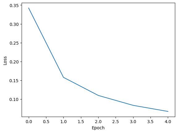
Epoch  1/5: 100%|██████████| 938/938 [00:34<00:00, 27.42it/s, train_loss=0.342]
Epoch  2/5: 100%|██████████| 938/938 [00:32<00:00, 28.44it/s, train_loss=0.158]
Epoch  3/5: 100%|██████████| 938/938 [00:33<00:00, 28.29it/s, train_loss=0.11]
Epoch  4/5: 100%|██████████| 938/938 [00:33<00:00, 28.29it/s, train_loss=0.0836]
Epoch  5/5: 100%|██████████| 938/938 [00:32<00:00, 28.54it/s, train_loss=0.0674]
The .fit method records the training loss for each epoch. The values are stored in the dictionary returned by the method, under the key 'train_loss'. We can plot them to visualize the training progress.
plt.plot(history['train_loss'])
plt.xlabel('Epoch')
plt.ylabel('Loss')
plt.show()