Model Architecture#
The multi-object localization model consists of two main components: a convolutional backbone for feature extraction and a localization head for bounding box prediction. The backbone is a pretrained convolutional network, such as MobileNetV3 or SSDLite, which can be run offline to extract features from images and store them on disk. This allows the localization head to be trained efficiently without repeatedly forwarding images through the backbone.
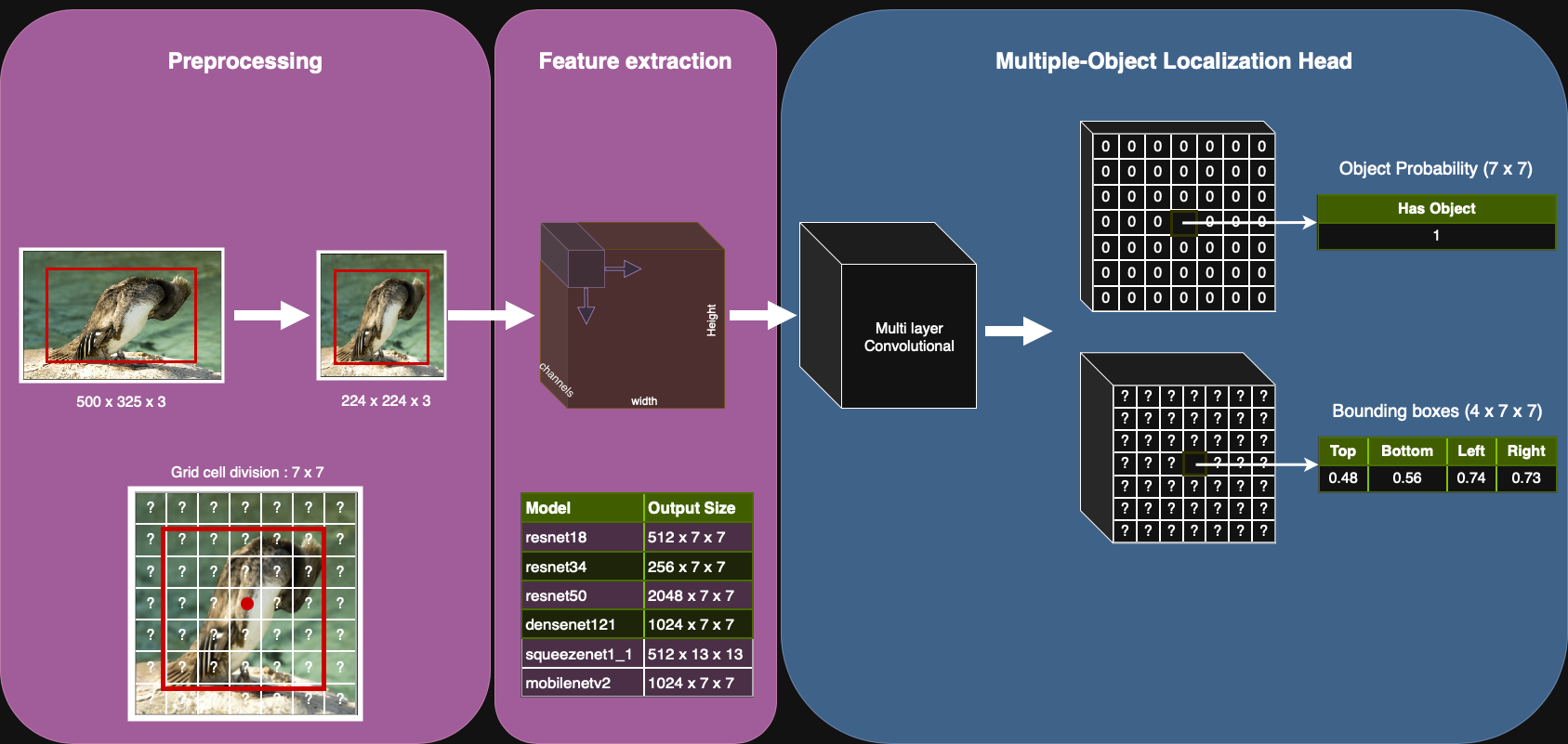
Localization Head#
The localization head operates directly on the spatial feature map produced by the backbone. It is structured as a small convolutional network with two parallel branches.
The classification branch predicts whether an object is present at each grid cell of the feature map. A minimal implementation uses a 1×1 convolutional layer with a single-output channel to produce a logit score for binary classification at each grid cell. More advanced setups use multiple stacked convolutions or larger kernels to incorporate context.
The regression branch predicts bounding box parameters for each grid cell. The simplest version again uses a 1×1 convolutional layer, but with as many output channels as there are bounding box parameters (see below). A deeper regression branch can improve localization accuracy.
Because the head is convolutional, the same weights are shared across the entire grid. This makes it possible to localize an arbitrary number of objects without knowing in advance how many there will be.
Design choices#
Kernel size. The simplest choice is to use 1×1 convolutions. This setup is easy to train and a good baseline. However, because each prediction only sees the features of a single cell, the model may struggle when an object spans multiple cells or when context is important. In such cases, the use of 3×3 convolutions with 1x1 padding allows the head to look at neighboring features, without changing the spatial dimensions of the feature map.
Branch depth. A shallow head is fast and works surprisingly well when the backbone already produces strong features. To get a working baseline, it is recommended to start with one or two convolutional layers per branch, and later experiment with deeper branches if needed.
Shared processing. In the simplest design, the classification and regression branches diverge immediately, each consisting of independent convolutional layers. Another option is to include a small “trunk” of shared layers before the split, so as to create common intermediate features. Sharing parameters in this way can improve efficiency and, in some cases, accuracy.
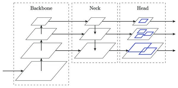
Multi-scale extension (optional)#
In the baseline architecture, the localization head is applied only to the deepest feature map produced by the backbone. While this is a reasonable starting point, it can struggle with objects of very different sizes. Specialized backbones, such as SSDLite, produce features at multiple scales to help mitigate such an issue.
To leverage multi-scale features effectively, they are often combined with a Feature Pyramid Network (FPN) immediately after the backbone. The localization head is then applied independently to each scale, and predictions from all heads are merged during inference. This produces an increased number of candidate boxes and improves detection across a wider range of object sizes.
Bounding box parametrization#
The regression branch does not predict raw pixel coordinates directly. Instead, it outputs bounding boxes in a different parametrization that is easier to learn. During training, these predictions may either be compared directly to ground-truth targets (encoded into the same parametrization), or decoded back into bounding box coordinates for loss functions that operate on box geometry. During inference, decoding is always required to obtain final bounding box predictions. In what follows, we describe the parametrization used by anchor-free detectors (FCOS, YOLOv6, …), since this project does not make use of anchor boxes.
Notation |
Description |
|---|---|
\((W, H)\) |
Image size in pixels. |
\((S, S)\) |
Grid resolution. |
\((W/S, H/S)\) |
Cell size in pixels (stride). |
\((i, j)\) |
Row and column indices of the cell containing an object, where \(0 ≤ i, j < S\). |
\((x_{min}, y_{min}, x_{max}, y_{max})\) |
Pixel coordinates of the top-left and bottom-right corners of a bounding box. |
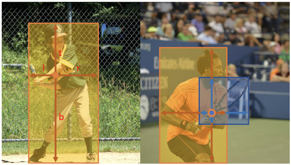
Encoding#
In anchor-free detectors, a bounding box is encoded by the distances from a cell center to the box edges. For a cell at row \(i\) and column \(j\), the pixel coordinates of its center are the following.
The bounding box coordinates are subtracted to/from the cell center to obtain the distances in pixels.
The figure below illustrates how these distances are defined. (When the cell center lies inside the bounding box, all four distances are nonnegative. If the center falls outside, some distances may become negative.)
Decoding#
The regression branch predicts the encoded distances \((\hat{l}, \hat{t}, \hat{r}, \hat{b})\) for each grid cell, without applying any activation function. As noted earlier, these predictions can be either compared directly against encoded ground-truth targets, or decoded into bounding box coordinates, depending on the loss function used. The decoding process simply reverses the above transformations to recover bounding box coordinates.
Normalized coordinates
The above formulas assume that all quantities are expressed in pixel units. In practice, it is often preferable to work with values that are normalized in the range [0,1]. This can be done as follows.
Case 1: Ground-truth bounding boxes are given in pixel coordinates.
After encoding, divide \(l\) and \(r\) by \(W\) and \(t\) and \(b\) by \(H\) to get normalized distances.
Before decoding, multiply \(\hat{l}\) and \(\hat{r}\) by \(W\) and \(\hat{t}\) and \(\hat{b}\) by \(H\) to recover pixel distances.
If you want decoding to yield normalized coordinates instead, keep distances normalized and divide the cell center \((g_x, g_y)\) by \((W, H)\).
Case 2: Ground-truth bounding boxes are given in normalized coordinates.
Use normalized cell centers \((g_x/W, g_y/H)\) in both encoding and decoding.
To recover pixel coordinates after decoding, multiply \(x_{min}, x_{max}\) by \(W\) and \(y_{min}, y_{max}\) by \(H\).
Implementation advice#
Keeping data transformations separate from the model makes it easier to experiment with different parametrizations and loss functions. The regression branch always outputs encoded values, but the model itself does not perform any encoding or decoding. If the chosen loss function operates on encoded values, the ground-truth boxes can be encoded either during preprocessing or inside the loss function. When bounding box coordinates are required, the model predictions can be decoded on-the-fly within the loss function. By maintaining a clear separation, you can revisit design choices without altering the network.