Evaluating a Neural Network#
Evaluating a neural network is as important as designing and training it, arguably more so when the predictions are to be trusted. Evaluation is a multifaceted process that requires careful consideration of various aspects. This includes understanding how the model behaves under different conditions, identifying potential failure modes, measuring latency and resource needs, and ensuring that the training process itself is functioning correctly. In this tutorial, we will be exclusively focused on evaluating the performance of a trained model on unseen data, using metrics that are appropriate for the task at hand.
Introduction#
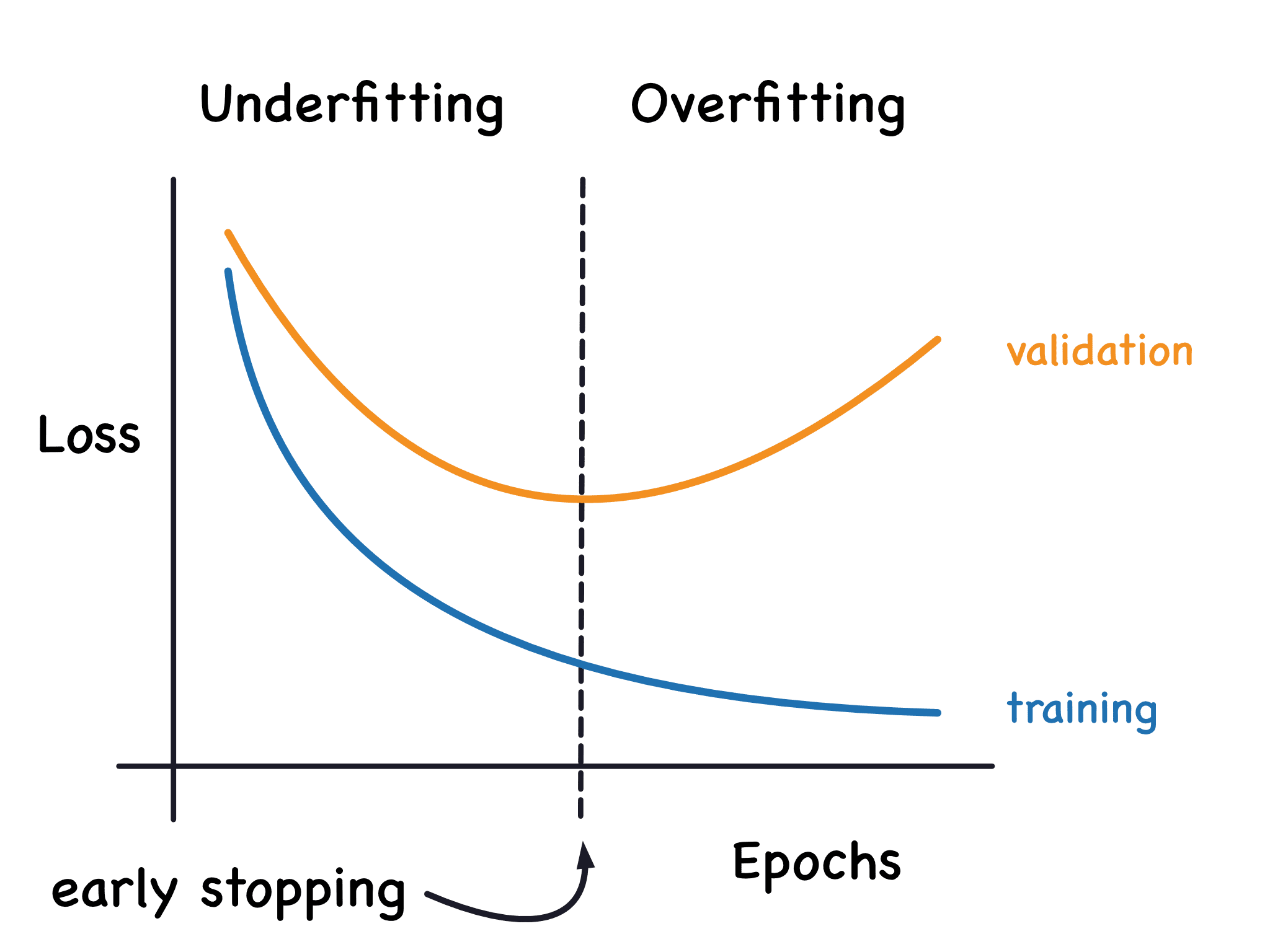
The fundamental challenge in machine learning is to balance the tension between optimization and generalization. Optimization is the process of adjusting a model so that it performs well on training data. By contrast, generalization refers to how well the trained model would perform on data it has never seen before. The ultimate goal of learning is to find a model that generalizes well. But the only aspect we can directly control is optimization. The more we optimize, the more the model learns to perform very well on the training data, but not necessarily on unseen data. This creates a tension that is inherent to the learning process.
A model that performs well on the training data but poorly on unseen data is said to be overfitting. Overfitting occurs when a model tends to memorize the training data, rather than learning the underlying patterns that would allow it to generalize to new data. This can be driven by many concrete causes, including excessive parameterization, systematic label noise, or simply a lack of diverse training examples.
To detect overfitting, it is essential to evaluate the model on data that was not used during training. This is why having a separate validation set is crucial. If the training loss keeps decreasing while the validation loss stalls or increases, the model is likely overfitting. Plotting learning curves makes this divergence visible and helps identify the point where early stopping would be beneficial. The key takeaway is that model evaluation is a crucial part of the training process that cannot be overlooked.
Evaluation metrics#
While PyTorch provides a robust framework for building and training models, it does not include built-in support for evaluation metrics like accuracy, precision, recall, etc. This omission can be inconvenient, as implementing metrics manually is time-consuming and error-prone. Fortunately, several third-party libraries have been developed to provide ready-to-use metrics implementations, such as Scikit-Learn, TorchMetrics, and TorchEval. In this book, we will use TorchEval for our evaluation needs.
Note
If you followed the instructions to set up your environment, you already have torcheval installed.
TorchEval#
TorchEval is a library developed by the PyTorch team that provides a variety of evaluation metrics for classification, regression, and other common tasks. It is designed to have two interfaces for each metric.
A functional API that computes the metric in a single call (stateless).
A class-based API that maintains state across multiple calls, allowing for incremental updates.
Both approaches are briefly demonstrated below.
Functional API#
The functional API in TorchEval allows you to compute metrics in a single call without maintaining any state. This is useful for quick evaluations on small datasets, or when you don’t need to keep track of intermediate results. Here’s an example of how to use the functional API to compute binary accuracy.
Show code cell source
import torch
from torcheval.metrics.functional import binary_accuracy

y_pred = torch.tensor([0, 1, 0, 1]) # Predicted labels
y_true = torch.tensor([0, 1, 1, 1]) # True labels

accuracy = binary_accuracy(y_pred, y_true)

assert accuracy == torch.mean((y_pred == y_true).float())
Binary Accuracy
The binary accuracy metric can handle several prediction formats.
Binary class labels
Probabilities
Logits
This is possible because the metric applies a threshold to the predictions. The default threshold is 0.5, but it can be adjusted by passing the threshold argument to the function or class constructor.
Class-based API#
The class-based API in TorchEval allows you to create metric objects that maintain state across multiple calls. This is useful for evaluating metrics over large datasets or when you want to keep track of intermediate results. Stateful metrics include three important methods.
reset(): Reset the metric to its initial state, preparing it for a new evaluation run.update(): Update the metric with new data (e.g., predictions and targets). This method is called for each mini-batch during evaluation.compute(): Compute the metric value by aggregating the data accumulated from previousupdate()calls. This method is called at the end of an evaluation run.
Here’s an example of how to use the class-based API to compute multiclass accuracy.
Show code cell source
import torch
from torcheval.metrics import MulticlassAccuracy

all_pred = torch.tensor([
    [2, 0, 1, 0],  # 1st batch
    [0, 2, 1, 1],  # 2nd batch
    [1, 0, 2, 1],  # 3rd batch
])
all_true = torch.tensor([
    [2, 0, 1, 1],  # 1st batch
    [0, 1, 2, 1],  # 2nd batch
    [1, 0, 2, 0],  # 3rd batch
])

metric = MulticlassAccuracy()

metric.reset()
for pred, true in zip(all_pred, all_true):
    metric.update(pred, true)
accuracy = metric.compute()

assert accuracy == torch.mean((all_pred == all_true).float())
Multiclass Accuracy
The multiclass accuracy metric can handle several prediction formats.
Integer class labels with shape (n_sample, )
Probabilities or logits with shape (n_sample, n_class)
This is possible because the metric applies an argmax(dim=1) operation to the predictions when they are passed to it as 2D tensors.
Evaluation loop#
The main purpose of the evaluation loop is to assess the model’s performance on a validation or test dataset. The evaluation loop is similar to the training loop, but with some important differences.
The model is set to evaluation mode, so that dropout and batch normalization layers are not updated.
The model is run inside a
torch.inference_mode()context to disable gradient computation.Task-specific metrics are evaluated instead of the loss function.
The following code snippet implements a minimal evaluation loop using TorchEval for metrics computation.
Show code cell source
import torch
from torch.utils.data import DataLoader
from torcheval.metrics import Metric


@torch.inference_mode()
def evaluation_loop(model: torch.nn.Module,
                    loader: DataLoader,
                    metrics: dict[str, Metric]) -> dict:

    # Device transfer
    device = torch.device("cuda" if torch.cuda.is_available() else "cpu")
    model.to(device)

    # Metric reset
    for metric in metrics.values():
        metric.reset()
        metric.to(device)

    # Evaluation mode
    model.eval()

    # Data iteration
    for inputs, labels in loader:

        # Forward pass
        inputs = inputs.to(device)
        labels = labels.to(device)
        outputs = model(inputs)

        # Metric update
        for metric in metrics.values():
            metric.update(outputs, labels)

    # Metric computation
    results = {name: metric.compute() for name, metric in metrics.items()}

    return results
Tip
The training.py script already includes an evaluation loop. Alternatively, for more control over the evaluation process, you can customize the evaluation_loop function defined above.
Complete learning pipeline#
Bringing everything together, we can now implement a complete learning pipeline that includes data loading, model definition, training, and evaluation. We start by importing PyTorch and all required modules, including the Trainer class from the training.py file.
import torch
from torch import nn, optim
from torch.utils.data import DataLoader
import torch.nn.functional as F
from torcheval.metrics import MulticlassAccuracy, MulticlassConfusionMatrix
from torchvision.transforms import v2
from torchvision.datasets import MNIST
import matplotlib.pyplot as plt
from training import Trainer
Dataset#
As a first step, we load the MNIST dataset with a preprocessing that converts the images into PyTorch tensors and normalizes their values to the range [0, 1]. We also create a DataLoader for the training set, and a separate DataLoader for the test set, which we will use for validation.
preprocess = v2.Compose([v2.ToImage(), v2.ToDtype(torch.float32, scale=True)])

train_ds = MNIST('.data', train=True,  download=True, transform=preprocess)
test_ds  = MNIST('.data', train=False, download=True, transform=preprocess)

train_loader = DataLoader(train_ds, batch_size=64, shuffle=True)
test_loader  = DataLoader(test_ds,  batch_size=256, shuffle=False)
Model#
Then, we define a simple feedforward neural network for classifying the MNIST images.
class SimpleNet(nn.Module):

    def __init__(self, input_dim, num_classes):
        super().__init__()
        self.flatten = nn.Flatten()
        self.linear1 = nn.Linear(input_dim, 512)
        self.linear2 = nn.Linear(512, num_classes)

    def forward(self, x):
        y = self.flatten(x)
        y = self.linear1(y)
        y = F.relu(y)
        y = self.linear2(y)
        return y
Training#
Next, we instantiate the model, the optimizer and the loss function. We create a Trainer object and register the multiclass accuracy as the metric we want to monitor during training. Then, we call the .fit method to train the model for a few epochs, using the test set for evaluation during the training process.
model = SimpleNet(28*28, 10)
optimizer = optim.Adam(model.parameters(), lr=1e-3)

loss_fn = nn.CrossEntropyLoss()
epochs = 5

trainer = Trainer()
trainer.set_metrics(accuracy=MulticlassAccuracy())

history = trainer.fit(model, train_loader, loss_fn, optimizer, epochs, test_loader)
===== Training on mps device =====
Epoch  1/5: 100%|██████████| 938/938 [00:36<00:00, 25.99it/s, accuracy=0.9612, train_loss=0.2609, valid_loss=0.1307]
Epoch  2/5: 100%|██████████| 938/938 [00:33<00:00, 28.16it/s, accuracy=0.9745, train_loss=0.1023, valid_loss=0.0833]
Epoch  3/5: 100%|██████████| 938/938 [00:32<00:00, 28.73it/s, accuracy=0.9758, train_loss=0.0643, valid_loss=0.0738]
Epoch  4/5: 100%|██████████| 938/938 [00:33<00:00, 28.18it/s, accuracy=0.9779, train_loss=0.0474, valid_loss=0.0687]
Epoch  5/5: 100%|██████████| 938/938 [00:34<00:00, 27.03it/s, accuracy=0.9790, train_loss=0.0329, valid_loss=0.0656]
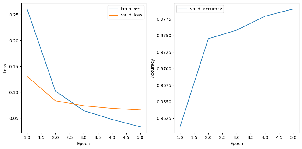
The loss function and all the validation metrics are recorded during training and returned in a dictionary. We can plot them to visualize the model performance over time. By inspecting the learning curves, we can see that the validation loss stalls after a few epochs, while the training loss continues to decrease. This indicates that the model is starting to overfit and more training would not improve its performance on unseen data.
Show code cell source
plt.figure(figsize=(10, 5), tight_layout=True)
plt.subplot(1, 2, 1)
plt.plot(range(1, epochs+1), history['train_loss'], label='train loss')
plt.plot(range(1, epochs+1), history['valid_loss'], label='valid. loss')
plt.xlabel('Epoch')
plt.ylabel('Loss')
plt.legend()
plt.subplot(1, 2, 2)
plt.plot(range(1, epochs+1), history['accuracy'], label='valid. accuracy')
plt.xlabel('Epoch')
plt.ylabel('Accuracy')
plt.legend()
plt.show()
Evaluation#
Finally, we evaluate the trained model on the test set to get an estimate of its performance on unseen data. We use the .eval method of the Trainer to run the evaluation loop and compute the metrics we registered earlier. The method returns a dictionary with the computed multiclass accuracy.
results = trainer.eval(model, test_loader)

print(f"Test accuracy: {results['accuracy']:.2%}")
Test accuracy: 97.90%
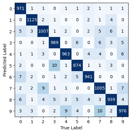
To evaluate the model on a different metric or dataset, we can reuse the existing Trainer. For example, the confusion matrix is a useful metric for classification tasks, as it provides a detailed breakdown of the model’s performance across different classes. Here’s how to compute the confusion matrix using TorchEval metrics.
# Sparse tensors not supported on MPS devices
if trainer._device.type == 'mps':
    trainer.to('cpu')

trainer.set_metrics(confmat=MulticlassConfusionMatrix(10))

results = trainer.eval(model, test_loader)
Show code cell source
confmat = results['confmat'].int()
num_classes = confmat.shape[0]

plt.imshow(confmat, cmap='Blues', norm=plt.Normalize(0, 30))
plt.xlabel('True Label')
plt.ylabel('Predicted Label')
plt.xticks(range(num_classes))
plt.yticks(range(num_classes))
for i in range(num_classes):
    for j in range(num_classes):
        plt.text(j, i, confmat[i, j].item(), ha='center', va='center', color='white' if i == j else 'black')
See also
A confusion matrix is a table that describes the performance of a classification model.
For binary classification, the confusion matrix is a 2x2 matrix that contains four values: true positive, true negative, false positive, and false negative.
For multi-class classification, the confusion matrix is an NxN matrix, where N is the number of classes. Each row represents the instances in a predicted class, while each column represents the instances in an actual class. The diagonal elements represent the number of correct predictions, while off-diagonal elements represent incorrect predictions.
Summary#
In this tutorial, we learned how to evaluate a neural network using the TorchEval library. We also implemented a complete learning pipeline, providing you with an overview of the entire deep learning workflow in PyTorch, from data loading to model evaluation. We hope this series of tutorials has given you a clear picture of how all the pieces fit together in a real-world PyTorch project.