Weak Supervision

Image retrieval aims to find images in a dataset that are visually or semantically similar to a query image. Deep metric learning has proven effective for this task by mapping images into an embedding space where simple distance metrics reflect semantic similarity. Traditionally, training such models requires large amounts of carefully annotated data. This is an expensive and time-consuming process that limits the applicability of this approach to many real-world scenarios.

Weak supervision offers a compelling alternative by using less precise labels to guide the learning process. Instead of requiring exact annotations for every class in the dataset or every object within an image, weak supervision makes use of broader information such as image-level tags or pairwise similarity judgments. These labels are often easier to collect and can reflect the ambiguity inherent in comparing images.

The Totally Looks Like dataset is an excellent example of a resource built around weak supervision. Rather than providing exhaustive labels, this dataset offers pairs of images that “look alike,” reflecting a natural notion of similarity as perceived by humans. These weakly annotated pairs serve as a valuable signal for training a Siamese network with the triplet loss. By learning from such data, the network is encouraged to map visually similar images to nearby points in an embedding space, even when the supervisory signal is not as strong or explicit as fully-labeled classification datasets.

In this tutorial, we will demonstrate how to train a Siamese network using the triplet loss with weak supervision. We will use the Totally Looks Like dataset to train a model that can retrieve images that look alike. We will also show how to evaluate the model by computing the retrieval accuracy on a test set.

import torch
import torchvision.transforms.v2 as v2
from torchvision.models import mobilenet_v3_large, MobileNet_V3_Large_Weights
from sklearn.model_selection import train_test_split
import matplotlib.pyplot as plt
from PIL import Image
import os

Dataset

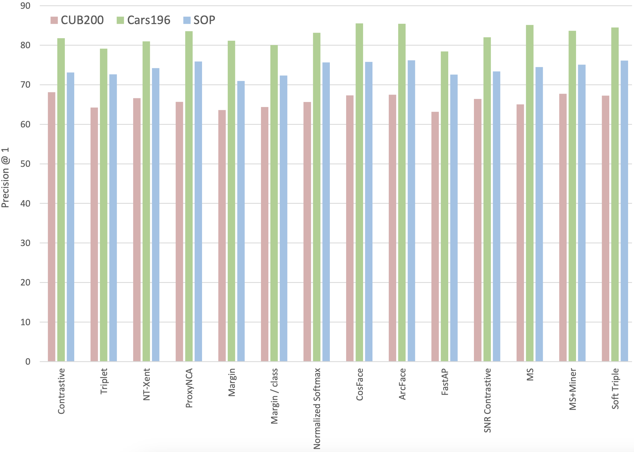
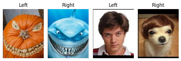
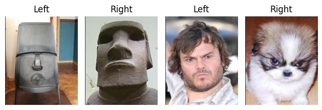
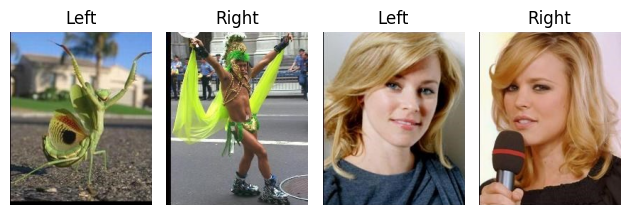
Totally-Looks-Like (TLL) is a dataset designed to reproduce human perception of image similarity. It is based on the similarly-named popular entertainment website. The dataset contains 6016 image pairs deemed to look alike by human annotators. The images are diverse and cover a wide range of categories, including objects, scenes, patterns, animals, and faces across various modalities (sketch, cartoon, natural images). We refer to the images in a pair as the “left image” and the “right image”.

The objective of this study is to assess to what degree a Siamese network can learn to retrieve images that look alike. For a given left image, we will measure the distance to all the right images using the learned embedding space. We will rank the right images by distance and evaluate the ranking by computing the retrieval accuracy.

Download the images

The dataset is available for download from the Totally Looks Like website. Unzip the downloaded file and look for the left.zip and right.zip archives. Extract the contents of these archives into a directory created alongside this notebook. The directory structure should look like this.

Totally-Looks-Like/
├── left/
│   ├── 0001.jpg
│   ├── 0002.jpg
│   └── ...
└── right/
    ├── 0001.jpg
    ├── 0002.jpg
    └── ...

Define a custom dataset

We create a custom dataset class to load the TLL images. The dataset constructor requires the path to the directory containing the left and right subdirectories. An optional transform argument can be passed to apply transformations to the images using the torchvision.transforms.v2 API. The __getitem__ method loads the pair of images corresponding to the given index and returns them as a tuple. The images are loaded using the Python Imaging Library (PIL) and converted to RGB. If any transformations are specified, they are applied to both images.

class TotallyLookLike(torch.utils.data.Dataset):

    def __init__(self, root, transform=None):
        self.root = root
        self.transform = transform
        self.left_dir = os.path.join(root, 'left')
        self.right_dir = os.path.join(root, 'right')
        self.filenames = sorted(os.listdir(self.left_dir))

    def __len__(self):
        return len(self.filenames)

    def __getitem__(self, idx):
        left = Image.open(os.path.join(self.left_dir, self.filenames[idx])).convert('RGB')
        right = Image.open(os.path.join(self.right_dir, self.filenames[idx])).convert('RGB')
        if self.transform:
            left = self.transform(left)
            right = self.transform(right)
        return left, right

Let’s create an instance of the TTL dataset and print its size.

dataset = TotallyLookLike('.data/Totally-Looks-Like/')

print('Number of image pairs:', len(dataset))

Number of image pairs: 6016

Visualize the image pairs

Let’s visualize a few image pairs from the dataset.

Show code cell source Hide code cell source

indices = [26, 1635, 65, 115, 123, 322, 133, 625]

for i in range(0, len(indices), 2):
    plt.figure(tight_layout=True)
    for j in range(2):
        anchors, positives = dataset[indices[i+j]]
        plt.subplot(1, 4, 1 + j*2)
        plt.imshow(anchors)
        plt.title('Left')
        plt.axis('off')
        plt.subplot(1, 4, 2 + j*2)
        plt.imshow(positives)
        plt.title('Right')
        plt.axis('off')
    plt.show()

Loss functions

The goal of weakly-supervised learning is to learn an embedding space where similar images (e.g., look-alike pairs) are close together, while dissimilar images are pushed apart. Two common loss functions used to enforce this structure are Triplet Loss and Normalized Temperature-scaled Cross-Entropy (NT‑Xent) Loss.

Triplet loss

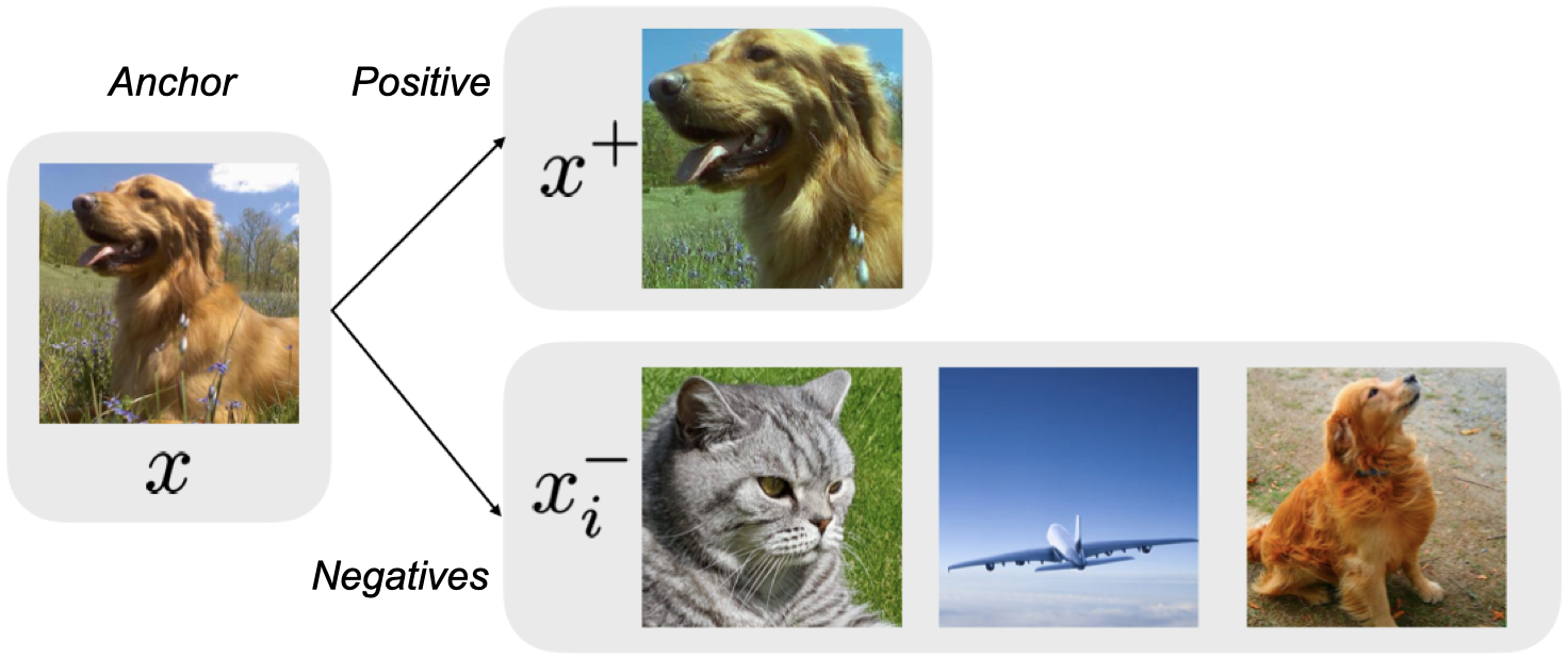
As discussed in the previous tutorial, Triplet loss operates on triplets consisting of an anchor, a positive, and a negative. Its objective is to ensure that the distance between the anchor and its positive is smaller than the distance between the anchor and any negative by at least a predefined margin. In the context of weak supervision, the positive pairs come directly from the dataset, while the negative pairs are sampled “online” from the current batch, using batch-hard or batch-all mining strategy.

The class below defines the triplet loss for a given batch of anchors and positives. Specifically, it computes the matrix of pairwise distances between the anchors and the positives, takes the diagonal elements as the anchor-positive distances, and the off-diagonal elements as the anchor-negative distances. The loss is then computed via broadcasting to ensure that each anchor-positive distance is compared to the distances of the same anchor with all the negatives.

class WeakTripletLoss(torch.nn.Module):
    """
    Triplet loss for weakly-supervised learning, using a batch-all negative mining strategy.
    """

    def __init__(self, margin=0.5):
        super().__init__()
        self.margin = margin

    def forward(self, anchors, positives):
        assert anchors.shape == positives.shape, 'Anchors and positives must have the same shape.'

        # Pairwise distances between embeddings
        distances = torch.cdist(anchors, positives, p=2)
        
        # The diagonal contains distances between each anchor and its true positive.
        anchor_positive_dist = distances.diag()
        
        # The off-diagonal elements contain the anchor-negative distances.
        diag_mask = torch.eye(anchors.size(0), dtype=torch.bool, device=anchors.device)
        anchor_negative_dist = distances.masked_fill(diag_mask, float('inf'))

        # Combine the anchor-positive distance to all the achor-negative distances
        loss = anchor_positive_dist.unsqueeze(1) - anchor_negative_dist + self.margin

        # Remove easy triplets
        loss = loss[loss > 0]

        # Handle case when all triplets are easy
        return loss.mean() if loss.numel() > 0 else torch.tensor(0.0, device=anchors.device)

NT-Xent loss

NT-Xent loss was introduced in 2016 as a generalization to the triplet loss that allows for the comparison of an anchor with multiple negatives. It is defined as the cross-entropy loss of an idealized task where the positive and negatives are treated as classes. Instead of the Euclidean distance, NT-Xent uses the cosine similarity to compare the anchor to the positive/negatives, normalized by a temperature parameter.

\[ \mathcal{L}_\text{NT-Xent}(z_i, z_j) = -\log\left(\frac{\exp(\text{sim}(z_i, z_j) / \tau)}{\sum_{k=1}^{N} \exp(\text{sim}(z_i, z_k) / \tau)}\right), \qquad \text{sim}(z_i, z_j) = \frac{z_i \cdot z_j}{\|z_i\| \|z_j\|}. \]

The class below defines the NT-Xent loss for a given batch of anchors and positives. It computes the cosine similarity between the anchors and the positives, builds the labels that assign each anchor to its positive, and then computes the cross-entropy loss. By its very definition, the NT-Xent loss adopts a batch-all mining strategy, where all the negatives are considered for each anchor.

class NTXentLoss(torch.nn.Module):
    """
    NT-Xent loss for weakly-supervised learning, using a batch-all negative mining strategy.
    """

    def __init__(self, temperature=0.5, normalize=False):
        super().__init__()
        self.temperature = temperature
        self.normalize = normalize

    def forward(self, anchors, positives):
        assert anchors.shape == positives.shape, 'Anchors and positives must have the same shape.'

        # Normalize the embeddings if needed
        if self.normalize:
            anchors   = torch.nn.functional.normalize(anchors, dim=-1)
            positives = torch.nn.functional.normalize(positives, dim=-1)

        # Each entry (i, j) is the cosine similarity between anchors[i] and positives[j]
        logits = anchors @ positives.T / self.temperature

        # For each i, anchor[i] is similar to positive[i] and dissimilar to all other positives.
        labels = torch.arange(anchors.size(0), device=anchors.device)

        # Compute the cross entropy loss, where each positive is treated as a class.
        return torch.nn.functional.cross_entropy(logits, labels)

Pretraining

Having defined the dataset and loss functions, the next step is to prepare the essential components that enable weakly-supervised training. We will extract features using a pre-trained backbone, organize these features into train and test sets, and define an embedding model that maps them into an embedding space.

MobileNet V3

We begin by extracting features from images using the backbone of a pre-trained model, such as MobileNet or ResNet. The pre-trained model is used solely as a feature extractor, and its classification head is removed or bypassed so that the output is a high-dimensional feature vector.

weights = MobileNet_V3_Large_Weights.DEFAULT
preprocess = weights.transforms()
mobilenet = mobilenet_v3_large(weights=weights)

The pre-trained model comes with its ows preprocessing pipeline, so we need to ensure that the input images are transformed accordingly.

dataset = TotallyLookLike('.data/Totally-Looks-Like/', transform=preprocess)

loader = torch.utils.data.DataLoader(dataset, batch_size=128, pin_memory=True)

Feature extraction

Now, we are ready to extract features from the TLL dataset using the pre-trained model. We will extract features for both the left and right images and store them in separate tensors.

device = torch.device('cuda' if torch.cuda.is_available() else 'mps' if torch.mps.is_available() else 'cpu')

mobilenet.eval()
mobilenet.to(device)

left_features = []
right_features = []

with torch.inference_mode():
    for left, right in loader:
        left = left.to(device)
        right = right.to(device)
        left_features.append(mobilenet.features(left).cpu())
        right_features.append(mobilenet.features(right).cpu())

left_features = torch.cat(left_features)
right_features = torch.cat(right_features)

print('Left features:', left_features.shape)
print('Right features:', right_features.shape)

Left features: torch.Size([6016, 960, 7, 7])
Right features: torch.Size([6016, 960, 7, 7])

Feature dataset

Once the features are extracted, it is necessary to organize them into a dataset that supports efficient data loading during training. We construct a custom PyTorch dataset that handles the pairing of pre-computed features corresponding to look-alike images. This dataset is designed to seamlessly supply the necessary inputs for the triplet loss or NT-Xent loss.

class FeatureDataset(torch.utils.data.Dataset):

    def __init__(self, left_features, right_features):
        self.left_features = left_features
        self.right_features = right_features

    def __len__(self):
        return len(self.left_features)

    def __getitem__(self, idx):
        return self.left_features[idx], self.right_features[idx]

We partition the dataset into training and test sets, and create datasets for both.

train_idx, test_idx = train_test_split(range(len(left_features)), test_size=0.2, shuffle=True, random_state=42)

train_ds = FeatureDataset(left_features[train_idx], right_features[train_idx])
test_ds  = FeatureDataset(left_features[test_idx],  right_features[test_idx])

Embedding head

The embedding head is a neural network that projects the high-dimensional feature vectors extracted by the pre-trained model into a lower-dimensional embedding space suitable for metric learning. This module typically consists of one or more fully connected layers, optionally followed by batch normalization and a non-linearity, with a final L2 normalization to enforce unit norm. Normalizing the embeddings is crucial for ensuring that the distance between embeddings is scale-invariant. It is also necessary for computing the cosine similarity in the NT-Xent loss.

class EmbeddingHead(torch.nn.Module):

    def __init__(self, in_dim, out_dim):
        super().__init__()
        self.head = torch.nn.Sequential(
            torch.nn.Flatten(),
            torch.nn.Linear(in_dim, 1024),
            torch.nn.ReLU(),
            torch.nn.Linear(1024, out_dim, bias=False),
            torch.nn.BatchNorm1d(out_dim)
        )

    def forward(self, x):
        x = self.head(x)
        x = torch.nn.functional.normalize(x, p=2, dim=1)
        return x

Training

With the dataset and loss functions in place, the next step is to train the embedding network under a weak supervision paradigm. In this section, we detail the training process, including setting up the training loop for weakly-supervised learning.

Train step

The training loop requires a function that performs a single optimization step on a batch of data. This function takes the feature tensors corresponding to the left and right images, computes the embeddings using the model, calculates the loss using the triplet loss or NT-Xent loss, and updates the model parameters via backpropagation. It is implemented below as the train_step function, which is designed to work with the generic training loop used in previous tutorials.

def train_step(model: torch.nn.Module, 
               batch: tuple[torch.Tensor, torch.Tensor],
               loss_fn: torch.nn.Module, 
               optimizer: torch.optim.Optimizer, 
               device: torch.device) -> float:
    
    # Unpack the batch
    left, right = batch

    # Send data to device
    left  = left.to(device)
    right = right.to(device)

    # Forward pass
    anchors   = model(left)
    positives = model(right)

    # Compute loss
    loss = loss_fn(anchors, positives)

    # Backward pass
    loss.backward()

    # Update model
    optimizer.step()
    optimizer.zero_grad()

    return loss.item()

Training loop

The training process begins by assembling the model. In our pipeline, the pre-extracted features are passed through an embedding head to obtain the final embedding representations. A DataLoader is used to handle batching with a large batch size. An optimizer is then defined to update the parameters of the embedding head. Depending on the chosen objective, one may use either Triplet Loss or NT‑Xent Loss.

import sys
sys.path.append('../../code')  # folder with train.py

from train import trainer

Show code cell source Hide code cell source

seed = 0
torch.manual_seed(seed)
if torch.mps.is_available():
    torch.mps.manual_seed(seed)
if torch.cuda.is_available():
    torch.cuda.manual_seed(seed)
    torch.cuda.manual_seed_all(seed)
    torch.backends.cudnn.deterministic = True
    torch.backends.cudnn.benchmark = False

cosine_similarity = False

model = EmbeddingHead(960*7*7, 128)
loader = torch.utils.data.DataLoader(train_ds, batch_size=512, pin_memory=True, shuffle=True)

optimizer = torch.optim.Adam(model.parameters(), lr=1e-3, amsgrad=True)

if cosine_similarity:
    loss_fn = NTXentLoss(0.1)
else:
    loss_fn = WeakTripletLoss(0.5)

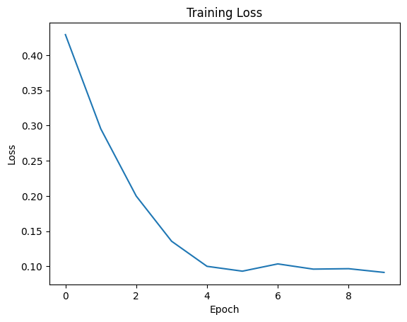
history = trainer(model, loader, loss_fn, optimizer, epochs=10, train_step=train_step)

===== Training on mps device =====

Epoch  1/10: 100%|██████████| 10/10 [00:04<00:00,  2.20it/s, train_loss=0.429]
Epoch  2/10: 100%|██████████| 10/10 [00:02<00:00,  3.42it/s, train_loss=0.295]
Epoch  3/10: 100%|██████████| 10/10 [00:02<00:00,  3.40it/s, train_loss=0.2]  
Epoch  4/10: 100%|██████████| 10/10 [00:02<00:00,  3.44it/s, train_loss=0.136]
Epoch  5/10: 100%|██████████| 10/10 [00:02<00:00,  3.41it/s, train_loss=0.1]  
Epoch  6/10: 100%|██████████| 10/10 [00:02<00:00,  3.44it/s, train_loss=0.0932]
Epoch  7/10: 100%|██████████| 10/10 [00:02<00:00,  3.43it/s, train_loss=0.103]
Epoch  8/10: 100%|██████████| 10/10 [00:02<00:00,  3.40it/s, train_loss=0.0961]
Epoch  9/10: 100%|██████████| 10/10 [00:02<00:00,  3.43it/s, train_loss=0.0967]
Epoch 10/10: 100%|██████████| 10/10 [00:02<00:00,  3.43it/s, train_loss=0.0914]

Show code cell source Hide code cell source

plt.plot(history['train'])
plt.xlabel('Epoch')
plt.ylabel('Loss')
plt.title('Training Loss')
plt.show()

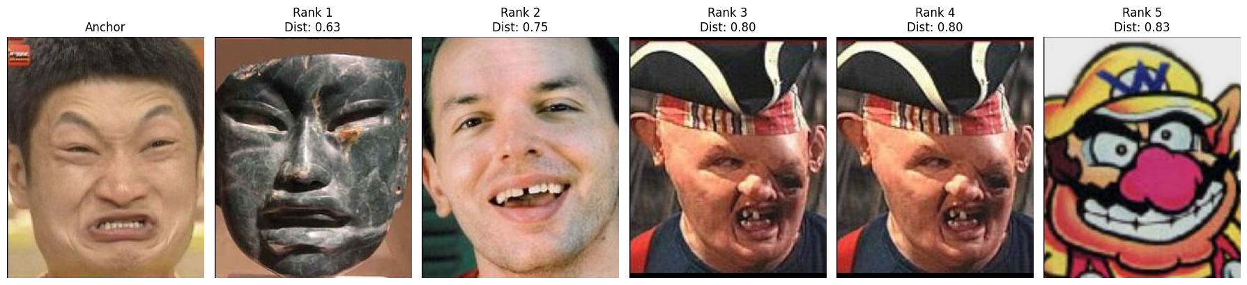
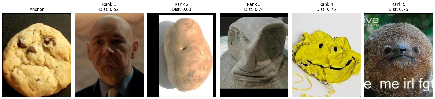
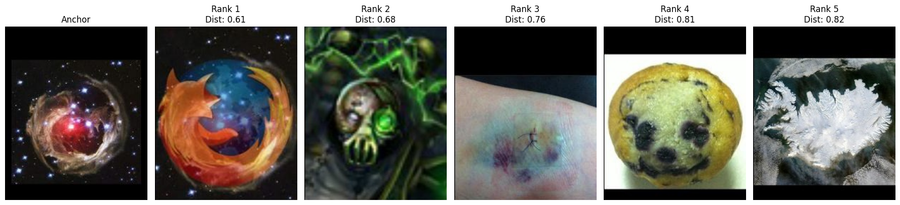
Evaluation

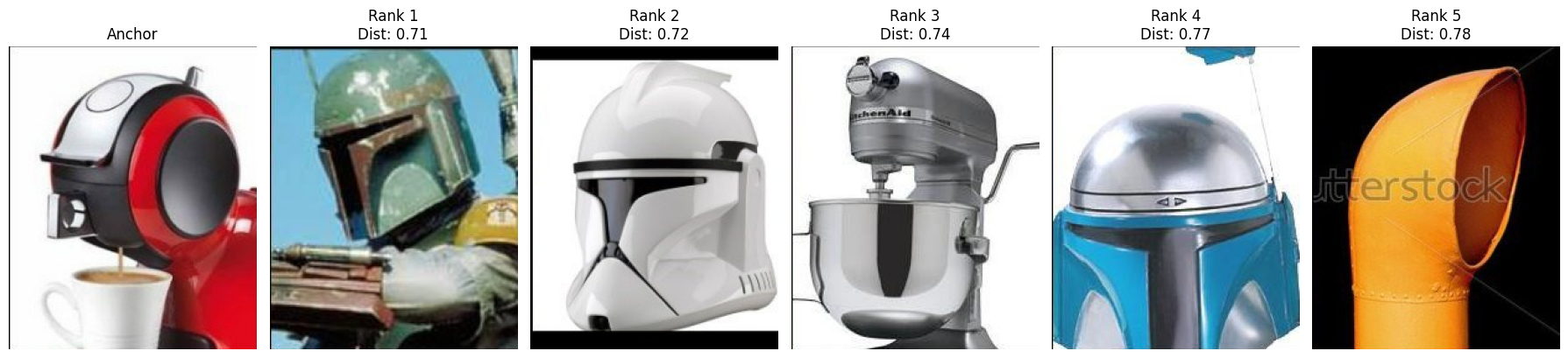
After training the model, we evaluate its ability to retrieve images that look alike. We will take a few left images from the test set and compute the distance to the right images of the whole dataset. We will rank the right images by distance and visualize the top-5 retrievals. We will then visually inspect the results to assess whether the model has learned to retrieve images that look alike.

Pairwise distances

The first step in evaluating the model is to compute the pairwise distances between the left and right images. To this end, we take the features extracted by the pre-trained model, pass them through the trained embedding head, and compute the pairwise distances between them.

model.eval()

# Embeddings
with torch.inference_mode():
    left_embeddings = model(left_features)
    right_embeddings = model(right_features)

# Distance matrix
if cosine_similarity:
    distances = 1 - left_embeddings @ right_embeddings.T
else:
    distances = torch.cdist(left_embeddings, right_embeddings, p=2)

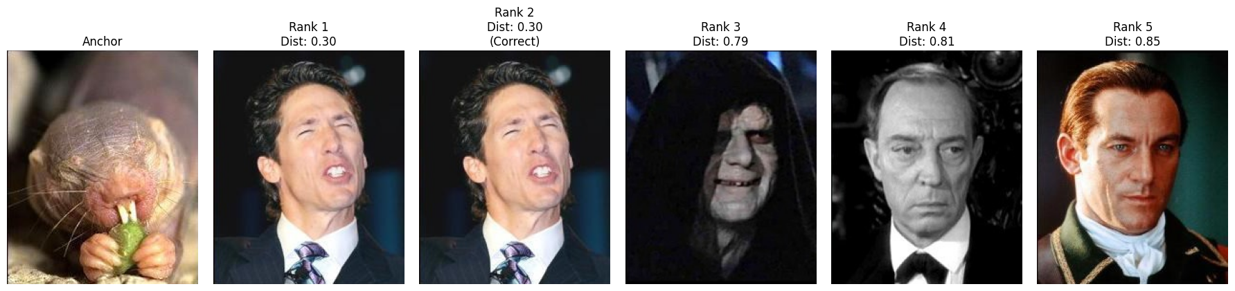
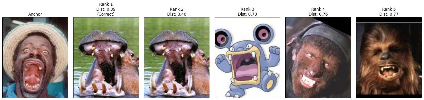
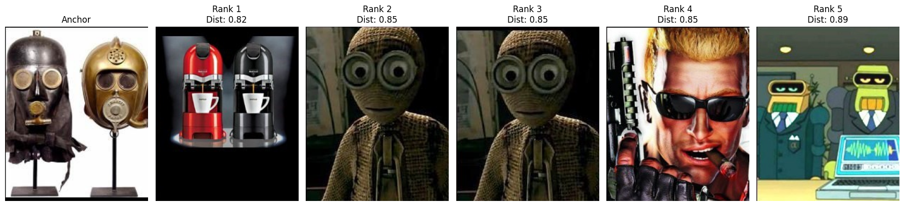
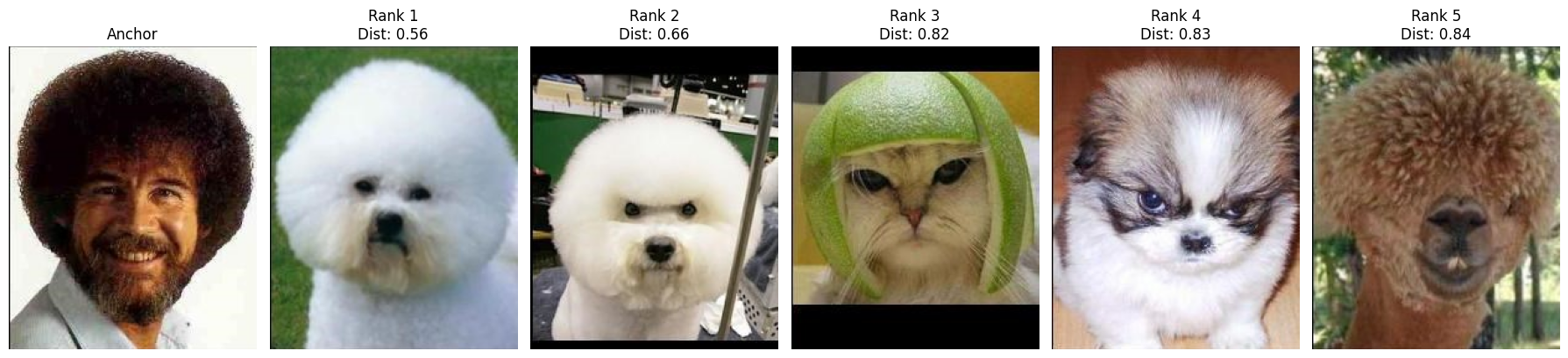
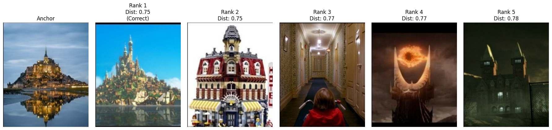
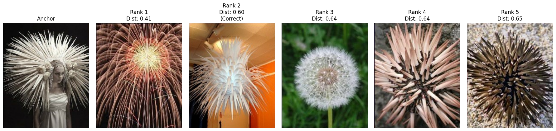
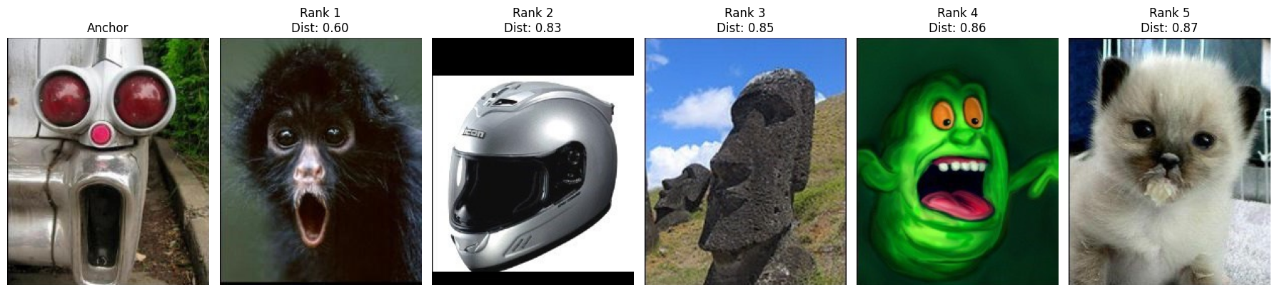
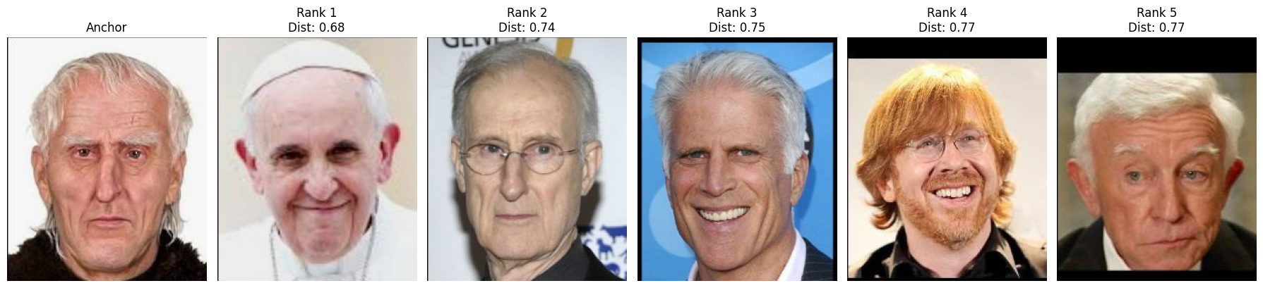
Top-5 retrieval

To illustrate the retrieval process, we select some query images and show the top-5 retrieved images.

Show code cell source Hide code cell source

def visualize_retrieval_results(anchor_index, distances, dataset, k=5):

    # Get the distance row for the selected anchor.
    anchor_distances = distances[anchor_index]
    
    # Since lower distances are better, sort in ascending order.
    topk = torch.topk(anchor_distances, k, largest=False)
    topk_indices = topk.indices.cpu().numpy()
    topk_values = topk.values.cpu().numpy()
    
    # Setup the plot: one column for the anchor and k columns for retrievals.
    fig, axes = plt.subplots(1, k+1, figsize=(3*(k+1), 4))
    
    # Plot the anchor image.
    left_image, _ = dataset[anchor_index]
    axes[0].imshow(left_image)
    axes[0].set_title("Anchor")
    axes[0].axis("off")
    
    # Plot the top-k retrieval results from the right folder.
    for i, (idx, dist_val) in enumerate(zip(topk_indices, topk_values), start=1):
        _, right_image = dataset[idx]
        axes[i].imshow(right_image)
        # You can also indicate if this is the correct match.
        label = f"Rank {i}\nDist: {dist_val:.2f}"
        if idx == anchor_index:
            label += "\n(Correct)"
        axes[i].set_title(label)
        axes[i].axis("off")
    
    plt.tight_layout()
    plt.show()

Show code cell source Hide code cell source

dataset = TotallyLookLike('.data/Totally-Looks-Like/')

for index in [102, 190, 379, 388, 465, 510, 876, 932, 1080, 1122, 1124, 1168]:
    anchor_index = test_idx[index]
    visualize_retrieval_results(anchor_index, distances, dataset)

Summary

In this tutorial, we explained how to train a Siamese network using triplet loss or NT-Xent loss with weak supervision. We used the Totally Looks Like dataset to train a model capable of retrieving visually similar images, and we validated the model performance by showing top‑5 retrievals for several query images.

Weak supervision offers a compelling alternative to traditional supervised learning by using less precise labels to guide the learning process. By learning from weakly annotated data, the network is encouraged to map visually similar images to nearby points in an embedding space, even when the supervisory signal is not as strong or explicit as fully-labeled classification datasets.

It is worth noting that while deep metric learning research over the past decade has frequently claimed significant advances, a closer examination reveals that such gains may be less substantial than reported. The study conducted by Musgrave et al. (2020) found that state-of-the-art loss functions perform marginally better than, and sometimes on par with, the triplet loss.