Data Augmentation#
Data augmentation is a technique used to artificially expand a training dataset by generating modified versions of existing data. In image processing, for example, new images can be created by applying transformations such as rotations, flips, or color adjustments. This approach acts as a simple yet powerful form of regularization that helps reduce overfitting by introducing more diversity into the training set. As a result, models trained with data augmentation tend to generalize better and perform more reliably on unseen data. This is especially valuable when the available dataset is limited or imbalanced. In this tutorial, we will demonstrate how to apply data augmentation to a simple CNN trained for image classification.
Show code cell source
import torch
import torch.nn.functional as F
import torchvision
import torchvision.transforms.v2 as v2

from sklearn.model_selection import train_test_split
import matplotlib.pyplot as plt
import pathlib
Preparation#
In the previous tutorial, we have already downloaded and extracted the cats-vs-dogs dataset in the directory .data/cats_vs_dogs/PetImages. We will reuse this dataset with the same preprocessing steps.
Show code cell source
IMAGE_SIZE = 128

# Image preprocessing
preprocess = v2.Compose([
    v2.ToImage(),
    v2.Resize(IMAGE_SIZE),
    v2.CenterCrop(IMAGE_SIZE),
    v2.ToDtype(torch.float32, scale=True),
])

# Load the full dataset
data_path = pathlib.Path(".data") / "cats_vs_dogs" / "PetImages"
dataset = torchvision.datasets.ImageFolder(data_path, transform=preprocess)

# Split the indices
train_idx, test_idx = train_test_split(range(len(dataset)), stratify=dataset.targets, test_size=0.2, shuffle=True, random_state=42)

# Create the subsets
train_ds = torch.utils.data.Subset(dataset, train_idx)
test_ds  = torch.utils.data.Subset(dataset, test_idx)

print(f"Train set: {len(train_ds)}")
print(f"Test set: {len(test_ds)}")
Train set: 18737
Test set: 4685
We will train a simple convolutional network on the cats-vs-dogs dataset. It is the same model as in the previous tutorial. To make this tutorial self-contained, we will copy the code below. But this is not the best practice. You should define the neural network in a separate Python file and import it.
Show code cell source
class BaselineModel(torch.nn.Module):

    def __init__(self, image_size: int):
        super().__init__()
        ksize = 3
        self.conv1 = torch.nn.Conv2d(3, 32, ksize)
        self.conv2 = torch.nn.Conv2d(32, 64, ksize)
        self.conv3 = torch.nn.Conv2d(64, 128, ksize)
        self.conv4 = torch.nn.Conv2d(128, 128, ksize)
        flat_dim = self.__calc_dim(image_size)
        self.fc1 = torch.nn.Linear(flat_dim, 256)
        self.fc2 = torch.nn.Linear(256, 1)

    def forward(self, x):
        for conv in [self.conv1, self.conv2, self.conv3, self.conv4]:
            x = F.relu(conv(x))
            x = F.max_pool2d(x, 2)
        x = torch.flatten(x, 1)
        x = F.relu(self.fc1(x))
        x = self.fc2(x)
        return x

    def __calc_dim(self, input_dim: int):
        """Returns the tensor size after the flatten layer."""
        n = input_dim
        for conv in [self.conv1, self.conv2, self.conv3, self.conv4]:
            n = n - conv.kernel_size[0] + 1 # CONV output size
            n = n // 2                      # POOL output size
        dim = n * n * self.conv4.out_channels
        return dim
Transforms#
TorchVision provides a list of transforms that make it easy to manipulate images. These operations can be used to preprocess or augment images during training or inference of various computer vision tasks, such as image classification, detection, segmentation, video classification. Here are the key points to remember.
Transforms behave like a regular
torch.nn.Module(in fact, most of them are).Most transforms accept both PIL images and PyTorch tensors as input.
Tensor images are expected to be in channel-first format, i.e., with shape (Channels, Height, Width).
Most transforms accept a batch of tensor images with an arbitrary number of leading dimensions.
The expected range of the values of a tensor image is implicitly defined by the data type.
Tensor images with a
floatdata type are expected to have values in [0, 1].Tensor images with a
uint8data type are expected to have values in [0, 255].Tensor images with an integer data type are expected to have values in [0, MAX_VALUE].
A series of transforms can be chained together using the
Composeclass.
We already encountered several transforms in the previous tutorials. Perhaps the two most used transforms are ToImage and ToDtype. The first one converts a PIL image to a PyTorch tensor, whereas the second one converts the data type and range of a tensor.
See also
This example illustrates the effect of various transforms provided by TorchVision.
Augmentation pipeline#
In this tutorial, we will use an augmentation pipeline that includes the following transforms.
RandomResizedCrop- Crop a random portion of the input image and resize it to a given size. The crop has a random area no larger than the given size, and a random aspect ratio between 3/4 and 4/3.RandomHorizontalFlip- Horizontally flip the input image with a given probability.ColorJitter- Randomly change the brightness, contrast, saturation and hue of the input image.
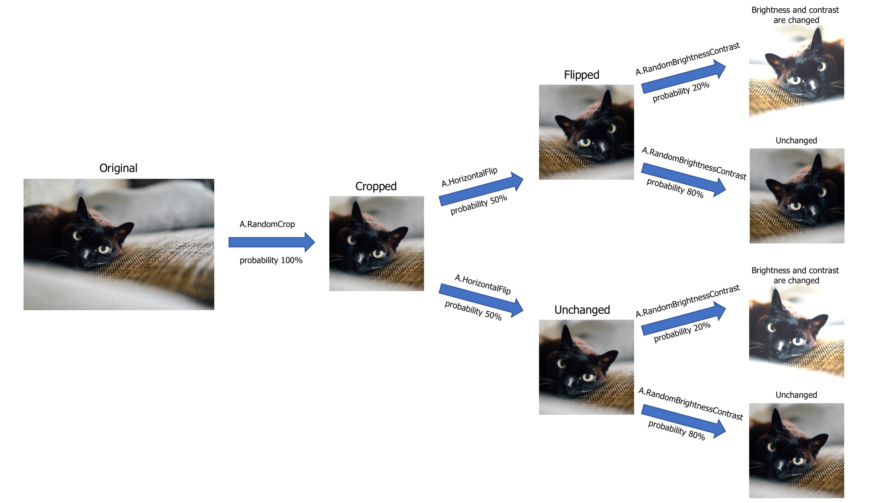
The figure below illustrates the augmentation pipeline that we are going to implement. Note that the horizontal flip and the color jitter are
skipped with a certain probability, based on a decision taken independently for each image in the batch. When a probability argument is not supported by a transform, which is the case for ColorJitter, we can use RandomApply to apply a transform with a given probability.
The code below defines the augmentation pipeline in PyTorch. Note that the pipeline includes the ToImage and ToDtype transforms. This ensures that the input to the neural network is a PyTorch tensor with floating-point values in [0, 1].
augmentation = v2.Compose([
    v2.ToImage(),
    v2.RandomResizedCrop(IMAGE_SIZE),
    v2.RandomHorizontalFlip(),
    v2.RandomApply([v2.ColorJitter(0.2, 0.2, 0.2, 0.2)], p=0.2),
    v2.ToDtype(torch.float32, scale=True)
])
Augmented training set#
At the beginning of this tutorial, we have created a training set without data augmentation. We will now create a training set that includes data augmentation. The test set will remain the same.
# Load the full dataset with augmentation
augmented_dataset = torchvision.datasets.ImageFolder(data_path, transform=augmentation)

# Create the train set using the same indices as before
augmented_train_ds = torch.utils.data.Subset(augmented_dataset, train_idx)
Note that ImageFolder use lazy loading, which means that the images are loaded on-the-fly when they are accessed. The augmentation is hence applied on-the-fly during training. This is called online data augmentation and is the most common way to apply data augmentation in deep learning.
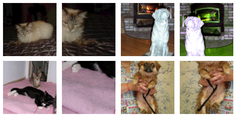
Visualizing the augmented images#
Let’s visualize some images from the augmented training set to see the effect of the augmentation pipeline.
Show code cell source
plt.figure(figsize=(8, 4), tight_layout=True)

for i in range(4):
    image, _ = train_ds[i]
    augmented, _ = augmented_train_ds[i]

    plt.subplot(2, 4, 1 + 2*i)
    plt.imshow(image.permute(1,2,0))
    plt.axis("off")
    plt.subplot(2, 4, 1 + 2*i + 1)
    plt.imshow(augmented.permute(1,2,0))
    plt.axis("off")
Training with data augmentation#
For completeness, we will now train the model on the augmented training set and evaluate it on the test set. (Reminder: the Trainer class is defined in the training.py file.)
from training import Trainer
from torcheval.metrics import BinaryAccuracy
Training uses the same hyperparameters as in the previous tutorial, with three minor differences.
We use the augmented training set.
We set
amsgrad=Truein the Adam optimizer.We train the model for more epochs on the augmented training set.
WARNING: The code below may take a long time to run without a GPU (about 3~4 minutes per epoch).
def loss_fn(output, target):
    return F.binary_cross_entropy_with_logits(output.squeeze(), target.float())

train_loader = torch.utils.data.DataLoader(augmented_train_ds, batch_size=64, shuffle=True)
test_loader  = torch.utils.data.DataLoader(test_ds, batch_size=128, shuffle=False)

model = BaselineModel(IMAGE_SIZE)
optimizer = torch.optim.Adam(model.parameters(), lr=0.0001, amsgrad=True)
epochs = 20

trainer = Trainer()
history = trainer.fit(model, train_loader, loss_fn, optimizer, epochs, test_loader)
===== Training on cuda device =====
Epoch  1/20: 100%|██████████| 293/293 [01:10<00:00,  4.16it/s, train_loss=0.6767, valid_loss=0.6364]
Epoch  2/20: 100%|██████████| 293/293 [01:15<00:00,  3.89it/s, train_loss=0.6513, valid_loss=0.6019]
Epoch  3/20: 100%|██████████| 293/293 [01:13<00:00,  4.01it/s, train_loss=0.6312, valid_loss=0.5926]
Epoch  4/20: 100%|██████████| 293/293 [01:13<00:00,  3.99it/s, train_loss=0.6180, valid_loss=0.5443]
Epoch  5/20: 100%|██████████| 293/293 [01:13<00:00,  3.99it/s, train_loss=0.6020, valid_loss=0.5258]
Epoch  6/20: 100%|██████████| 293/293 [01:13<00:00,  4.01it/s, train_loss=0.5852, valid_loss=0.5001]
Epoch  7/20: 100%|██████████| 293/293 [01:14<00:00,  3.93it/s, train_loss=0.5725, valid_loss=0.4848]
Epoch  8/20: 100%|██████████| 293/293 [01:13<00:00,  3.97it/s, train_loss=0.5567, valid_loss=0.4757]
Epoch  9/20: 100%|██████████| 293/293 [01:07<00:00,  4.32it/s, train_loss=0.5486, valid_loss=0.4511]
Epoch 10/20: 100%|██████████| 293/293 [01:18<00:00,  3.72it/s, train_loss=0.5352, valid_loss=0.4558]
Epoch 11/20: 100%|██████████| 293/293 [01:18<00:00,  3.73it/s, train_loss=0.5165, valid_loss=0.4308]
Epoch 12/20: 100%|██████████| 293/293 [01:24<00:00,  3.49it/s, train_loss=0.5164, valid_loss=0.4436]
Epoch 13/20: 100%|██████████| 293/293 [01:16<00:00,  3.81it/s, train_loss=0.5038, valid_loss=0.4233]
Epoch 14/20: 100%|██████████| 293/293 [01:15<00:00,  3.88it/s, train_loss=0.4928, valid_loss=0.4163]
Epoch 15/20: 100%|██████████| 293/293 [01:16<00:00,  3.85it/s, train_loss=0.4842, valid_loss=0.4023]
Epoch 16/20: 100%|██████████| 293/293 [01:12<00:00,  4.04it/s, train_loss=0.4810, valid_loss=0.4007]
Epoch 17/20: 100%|██████████| 293/293 [01:10<00:00,  4.14it/s, train_loss=0.4774, valid_loss=0.3877]
Epoch 18/20: 100%|██████████| 293/293 [01:10<00:00,  4.17it/s, train_loss=0.4704, valid_loss=0.3734]
Epoch 19/20: 100%|██████████| 293/293 [01:11<00:00,  4.09it/s, train_loss=0.4651, valid_loss=0.3673]
Epoch 20/20: 100%|██████████| 293/293 [01:10<00:00,  4.16it/s, train_loss=0.4601, valid_loss=0.3723]
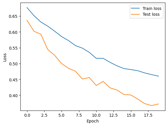
Let’s plot the loss of the model computed on the training and test sets.
Show code cell source
plt.plot(history['train_loss'], label='Train loss')
plt.plot(history['valid_loss'], label='Test loss')
plt.xlabel('Epoch')
plt.ylabel('Loss')
plt.legend()
plt.show()
Finally, we will evaluate the model on the test set and print the classification accuracy.
Show code cell source
from training import ModelAdapter

adapter = ModelAdapter(lambda x: x.squeeze())
trainer.set_adapter(adapter)

trainer.set_metrics(accuracy=BinaryAccuracy())
ans = trainer.eval(model, test_loader)

print(f"Test Accuracy: {ans['accuracy']:.2%}")
Test Accuracy: 84.06%
Summary#
In this notebook, we have learned how to use data augmentation in PyTorch. We have seen how to create an augmentation pipeline and apply it to a subset of the available data. We have also trained a simple CNN model on the cats-vs-dogs dataset using data augmentation.
Important
Data augmentation is applied dinamically during training. The images are transformed “on-the-fly” when a batch is sampled from the dataset. As a result, the model sees a different transformation of the images at each epoch, and the augmentations are never saved to disk.
Data augmentation is a powerful technique to increase the diversity of the training data and improve the generalization of the model. However, it is important to be careful with the choice of transformations, as some of them may not be suitable for the problem at hand. For example, flipping an image horizontally may not be a good idea for a dataset of handwritten digits. PyTorch provides a wide range of transformations that can be combined to create complex augmentation pipelines. But if you need more advanced augmentations, you can use specialized libraries like Albumentations.
You may still be wondering, “How do people who train state-of-the-art models use image augmentation?” The following table shows the data augmentation techniques used in some popular models.
Model |
Data Augmentations |
|---|---|
LeNet-5 |
Translate, Scale, Squeeze, Shear |
AlexNet |
Translate, Flip, Intensity Changing |
ResNet |
Crop, Flip |
DenseNet |
Flip, Crop, Translate |
MobileNet |
Crop, Elastic distortion |
NasNet |
Cutout, Crop, Flip |
ResNeSt |
AutoAugment, Mixup, Crop |
DeiT |
AutoAugment, RandAugment, Random erasing, Mixup, CutMix |
Swin Transformer |
RandAugment, Mixup, CutMix, Random erasing |
U-Net |
Translate, Rotate, Gray value variation, Elastic deformation |
Faster R-CNN |
Flip |
YOLO |
Scale, Translate, Color space |
SSD |
Crop, Resize, Flip, Color Space, Distortion |
YOLOv4 |
Mosaic, Distortion, Scale, Color space, Crop, Flip, Rotate, Random erase, Cutout, Hide and Seek, GridMask, Mixup, CutMix, StyleGAN |