Fine Tuning#
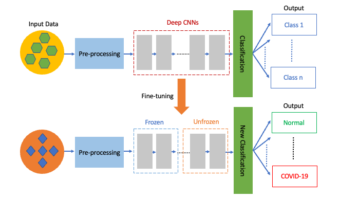
Fine tuning is the most common incarnation of transfer learning in the context of deep learning. It consists of taking a model that has been trained on a large dataset, such as ImageNet, and adapting its architecture and parameters to a new, smaller dataset. The key idea is that the lower layers of a convolutional network learn general features like edges and textures, while the higher layers capture more task-specific details. By freezing the lower layers and retraining only the upper layers on new data, we can achieve high performance with limited data and training time.
Effectively fine-tuning a convolutional network requires an understanding of pre-trained architectures, layer freezing, learning rate adjustments, and dataset-specific adaptations. In this tutorial, we will walk through the fine-tuning process, covering how to modify the architecture of a pre-trained model, and optimize its training strategy for a new task.
Model preparation#
Before we can dive into fine-tuning, we need to understand how to freeze layers and modify the architecture of a pre-trained model. We will illustrate these concepts by working with the MobileNetV3 architecture. As discussed in the previous tutorial, MobileNetV3 consists of three modules.
features- A series of convolutional and pooling layers to learn a representation of the input image.avgpool- A layer that averages the channels of the input 3D tensor to produce a feature vector.classifier- A series of fully-connected layers that predicts the class logits from the feature vector.
Let’s start by instanciating the MobileNetV3 model with randomly initialized weights.
Show code cell source
import torch
from torch import nn
from torchvision.models import mobilenet_v3_large, MobileNet_V3_Large_Weights
from torchinfo import summary
architecture = mobilenet_v3_large()
Trainable layers#
We can inspect the number of trainable tensors in a model by iterating through the model’s parameters and counting how many of them have requires_grad set to True. Alternatively, we can use the torchinfo package to get a summary of the model architecture, including the number of parameters and which ones are trainable. Let’s have an overview of the first two levels of the model. By default, all layers are trainable.
Show code cell source
summary(architecture, depth=2, col_names=["num_params", "trainable"])
====================================================================================================
Layer (type:depth-idx)                             Param #                   Trainable
====================================================================================================
MobileNetV3                                        --                        True
├─Sequential: 1-1                                  --                        True
│    └─Conv2dNormActivation: 2-1                   464                       True
│    └─InvertedResidual: 2-2                       464                       True
│    └─InvertedResidual: 2-3                       3,440                     True
│    └─InvertedResidual: 2-4                       4,440                     True
│    └─InvertedResidual: 2-5                       10,328                    True
│    └─InvertedResidual: 2-6                       20,992                    True
│    └─InvertedResidual: 2-7                       20,992                    True
│    └─InvertedResidual: 2-8                       32,080                    True
│    └─InvertedResidual: 2-9                       34,760                    True
│    └─InvertedResidual: 2-10                      31,992                    True
│    └─InvertedResidual: 2-11                      31,992                    True
│    └─InvertedResidual: 2-12                      214,424                   True
│    └─InvertedResidual: 2-13                      386,120                   True
│    └─InvertedResidual: 2-14                      429,224                   True
│    └─InvertedResidual: 2-15                      797,360                   True
│    └─InvertedResidual: 2-16                      797,360                   True
│    └─Conv2dNormActivation: 2-17                  155,520                   True
├─AdaptiveAvgPool2d: 1-2                           --                        --
├─Sequential: 1-3                                  --                        True
│    └─Linear: 2-18                                1,230,080                 True
│    └─Hardswish: 2-19                             --                        --
│    └─Dropout: 2-20                               --                        --
│    └─Linear: 2-21                                1,281,000                 True
====================================================================================================
Total params: 5,483,032
Trainable params: 5,483,032
Non-trainable params: 0
====================================================================================================
Freezing layers#
To freeze a layer, we set the requires_grad attribute to False for all parameters in that layer. This prevents the optimizer from updating the weights of the layer during training. We can use the parameters() iterator to access the parameters of a nn.Module and set the requires_grad attribute accordingly. The code below demonstrates how to freeze the convolutional backbone of MobileNetV3.
for params in architecture.features.parameters():
    params.requires_grad = False
Let’s regenerate the model summary after freezing the backbone. Only the parameters in the classification head should be trainable now.
Show code cell source
summary(architecture, depth=2, col_names=["num_params", "trainable"])
====================================================================================================
Layer (type:depth-idx)                             Param #                   Trainable
====================================================================================================
MobileNetV3                                        --                        Partial
├─Sequential: 1-1                                  --                        False
│    └─Conv2dNormActivation: 2-1                   (464)                     False
│    └─InvertedResidual: 2-2                       (464)                     False
│    └─InvertedResidual: 2-3                       (3,440)                   False
│    └─InvertedResidual: 2-4                       (4,440)                   False
│    └─InvertedResidual: 2-5                       (10,328)                  False
│    └─InvertedResidual: 2-6                       (20,992)                  False
│    └─InvertedResidual: 2-7                       (20,992)                  False
│    └─InvertedResidual: 2-8                       (32,080)                  False
│    └─InvertedResidual: 2-9                       (34,760)                  False
│    └─InvertedResidual: 2-10                      (31,992)                  False
│    └─InvertedResidual: 2-11                      (31,992)                  False
│    └─InvertedResidual: 2-12                      (214,424)                 False
│    └─InvertedResidual: 2-13                      (386,120)                 False
│    └─InvertedResidual: 2-14                      (429,224)                 False
│    └─InvertedResidual: 2-15                      (797,360)                 False
│    └─InvertedResidual: 2-16                      (797,360)                 False
│    └─Conv2dNormActivation: 2-17                  (155,520)                 False
├─AdaptiveAvgPool2d: 1-2                           --                        --
├─Sequential: 1-3                                  --                        True
│    └─Linear: 2-18                                1,230,080                 True
│    └─Hardswish: 2-19                             --                        --
│    └─Dropout: 2-20                               --                        --
│    └─Linear: 2-21                                1,281,000                 True
====================================================================================================
Total params: 5,483,032
Trainable params: 2,511,080
Non-trainable params: 2,971,952
====================================================================================================
Replacing layers#
Fine-tuning often requires modifying the architecture of the pre-trained model to adapt it to the new task. This can involve changing the number of output units in the classification head, adding new layers, or replacing existing layers. There are several ways to modify the architecture of a model in PyTorch. The simplest way is to just replace the layers in the classification head. For example, we can replace the two fully-connected layers of MobileNetV3 with new ones that have a different number of output units.
in_dim = architecture.classifier[0].in_features

architecture.classifier[0] = torch.nn.Linear(in_dim, 500)
architecture.classifier[3] = torch.nn.Linear(500, 1)  # binary classification
A more drastic approach is to replace the entire classification head with a new one. This can be done by creating a new nn.Module for the classification head, and replacing the classifier attribute of the model with the new module.
architecture.classifier = torch.nn.Sequential(
    torch.nn.Linear(in_dim, 500),
    torch.nn.ReLU(),
    torch.nn.Linear(500, 1)
)
Show code cell source
summary(architecture, depth=2, col_names=["num_params", "trainable"])
====================================================================================================
Layer (type:depth-idx)                             Param #                   Trainable
====================================================================================================
MobileNetV3                                        --                        Partial
├─Sequential: 1-1                                  --                        False
│    └─Conv2dNormActivation: 2-1                   (464)                     False
│    └─InvertedResidual: 2-2                       (464)                     False
│    └─InvertedResidual: 2-3                       (3,440)                   False
│    └─InvertedResidual: 2-4                       (4,440)                   False
│    └─InvertedResidual: 2-5                       (10,328)                  False
│    └─InvertedResidual: 2-6                       (20,992)                  False
│    └─InvertedResidual: 2-7                       (20,992)                  False
│    └─InvertedResidual: 2-8                       (32,080)                  False
│    └─InvertedResidual: 2-9                       (34,760)                  False
│    └─InvertedResidual: 2-10                      (31,992)                  False
│    └─InvertedResidual: 2-11                      (31,992)                  False
│    └─InvertedResidual: 2-12                      (214,424)                 False
│    └─InvertedResidual: 2-13                      (386,120)                 False
│    └─InvertedResidual: 2-14                      (429,224)                 False
│    └─InvertedResidual: 2-15                      (797,360)                 False
│    └─InvertedResidual: 2-16                      (797,360)                 False
│    └─Conv2dNormActivation: 2-17                  (155,520)                 False
├─AdaptiveAvgPool2d: 1-2                           --                        --
├─Sequential: 1-3                                  --                        True
│    └─Linear: 2-18                                480,500                   True
│    └─ReLU: 2-19                                  --                        --
│    └─Linear: 2-20                                501                       True
====================================================================================================
Total params: 3,452,953
Trainable params: 481,001
Non-trainable params: 2,971,952
====================================================================================================
Modifying the architecture#
The most general way to modify the architecture of a pre-trained model is to subclass nn.Module and redefine the forward method. This approach allows us to change the architecture in any way we want, including adding new layers, removing layers, or changing the connections between layers.
Important
Batch Normalization requires special handling during fine-tuning. These layers should be kept in evaluation mode and never be unfrozen (to retain pre-trained statistics and parameters).
To take into account the special handling of BatchNorm layers, we define four utility functions to make layers trainable or not, freeze layers by type, set layers of a certain type to evaluation mode, and unfreeze the last layers of a model. We will use these functions to prepare our model for fine-tuning.
Show code cell source
def make_trainable(model: nn.Module, grad: bool):
    """Set the requires_grad attribute of all parameters in a module"""
    for params in model.parameters():
        params.requires_grad = grad

def unfreeze_layers(model: nn.Sequential, count: int):
    """Unfreeze the last `count` layers of a Sequential model"""
    assert 0 <= count <= len(model)
    for layer in model[-count:]:
        make_trainable(layer, True)

def freeze_by_type(model: nn.Module, layer_type: type[nn.Module]|tuple[type[nn.Module]]):
    """Freeze the modules of a certain type"""
    for layer in model.modules():
        if isinstance(layer, layer_type):
            make_trainable(layer, False)

def set_eval_mode(model: nn.Module, layer_type: type[nn.Module]):
    """Set the modules of a certain type to evaluation mode"""
    for layer in model.modules():
        if isinstance(layer, layer_type):
            layer.eval()
Next, we define a new model that builds on the convolutional backbone of MobileNetV3. We replace the average pooling layer with a flattening operation, and we define a new classification head with two fully-connected layers. The first layer has 500 units and ReLU activation, while the second layer has a single output unit. We also provide utility methods to freeze and unfreeze the convolutional backbone.
class MobileNet(nn.Module):

    def __init__(self, weights: MobileNet_V3_Large_Weights = None):
        super().__init__()
        mobilenet = mobilenet_v3_large(weights=weights)
        self.backbone = mobilenet.features
        self.classifier = nn.Sequential(
            nn.Linear(960*7*7, 500),
            nn.ReLU(),
            nn.Linear(500, 1)
        )

    def forward(self, x):
        x = self.backbone(x)
        x = torch.flatten(x, 1)
        x = self.classifier(x)
        return torch.squeeze(x, -1)

    #----- Fine-tuning support -----#

    def train(self, mode: bool = True):
        """Set the model to training mode, except for BatchNorm layers"""
        super().train(mode)
        set_eval_mode(self.backbone, nn.BatchNorm2d)

    def freeze(self):
        """Freeze the backbone of the model"""
        make_trainable(self.backbone, False)

    def unfreeze(self, count: int):
        """Unfreeze the last layers of the backbone, except for BatchNorm layers"""
        unfreeze_layers(self.backbone, count)
        freeze_by_type(self.backbone, nn.BatchNorm2d)
Sanity check#
Let’s check that the model works as expected. First, we create an instance of the model and pass a random tensor through it to check the output shape. Like in the previous tutorial, the model output is squeezed so as to return a 1D tensor of shape (batch_size,) rather than a 2D tensor of shape (batch_size, 1).
batch = torch.rand(16, 3, 224, 224)

model = MobileNet()
output = model(batch)

assert output.shape == (16,)
Then, we freeze the convolutional backbone and check that only the classification head is trainable.
model.freeze()
Show code cell source
summary(model, depth=2, col_names=["num_params", "trainable"])
====================================================================================================
Layer (type:depth-idx)                             Param #                   Trainable
====================================================================================================
MobileNet                                          --                        Partial
├─Sequential: 1-1                                  --                        False
│    └─Conv2dNormActivation: 2-1                   (464)                     False
│    └─InvertedResidual: 2-2                       (464)                     False
│    └─InvertedResidual: 2-3                       (3,440)                   False
│    └─InvertedResidual: 2-4                       (4,440)                   False
│    └─InvertedResidual: 2-5                       (10,328)                  False
│    └─InvertedResidual: 2-6                       (20,992)                  False
│    └─InvertedResidual: 2-7                       (20,992)                  False
│    └─InvertedResidual: 2-8                       (32,080)                  False
│    └─InvertedResidual: 2-9                       (34,760)                  False
│    └─InvertedResidual: 2-10                      (31,992)                  False
│    └─InvertedResidual: 2-11                      (31,992)                  False
│    └─InvertedResidual: 2-12                      (214,424)                 False
│    └─InvertedResidual: 2-13                      (386,120)                 False
│    └─InvertedResidual: 2-14                      (429,224)                 False
│    └─InvertedResidual: 2-15                      (797,360)                 False
│    └─InvertedResidual: 2-16                      (797,360)                 False
│    └─Conv2dNormActivation: 2-17                  (155,520)                 False
├─Sequential: 1-2                                  --                        True
│    └─Linear: 2-18                                23,520,500                True
│    └─ReLU: 2-19                                  --                        --
│    └─Linear: 2-20                                501                       True
====================================================================================================
Total params: 26,492,953
Trainable params: 23,521,001
Non-trainable params: 2,971,952
====================================================================================================
Finally, we unfreeze some layers of the convolutional backbone and check that the corresponding parameters are trainable again, except for the BatchNorm layers. In the summary below, we can see that the last three layers of the backbone are marked as partially trainable, while the rest of the backbone remains frozen. Increasing the summary depth would show that the BatchNorm layers are still frozen, as expected.
model.unfreeze(3)
Show code cell source
summary(model, depth=2, col_names=["num_params", "trainable"])
====================================================================================================
Layer (type:depth-idx)                             Param #                   Trainable
====================================================================================================
MobileNet                                          --                        Partial
├─Sequential: 1-1                                  --                        Partial
│    └─Conv2dNormActivation: 2-1                   (464)                     False
│    └─InvertedResidual: 2-2                       (464)                     False
│    └─InvertedResidual: 2-3                       (3,440)                   False
│    └─InvertedResidual: 2-4                       (4,440)                   False
│    └─InvertedResidual: 2-5                       (10,328)                  False
│    └─InvertedResidual: 2-6                       (20,992)                  False
│    └─InvertedResidual: 2-7                       (20,992)                  False
│    └─InvertedResidual: 2-8                       (32,080)                  False
│    └─InvertedResidual: 2-9                       (34,760)                  False
│    └─InvertedResidual: 2-10                      (31,992)                  False
│    └─InvertedResidual: 2-11                      (31,992)                  False
│    └─InvertedResidual: 2-12                      (214,424)                 False
│    └─InvertedResidual: 2-13                      (386,120)                 False
│    └─InvertedResidual: 2-14                      (429,224)                 False
│    └─InvertedResidual: 2-15                      797,360                   Partial
│    └─InvertedResidual: 2-16                      797,360                   Partial
│    └─Conv2dNormActivation: 2-17                  155,520                   Partial
├─Sequential: 1-2                                  --                        True
│    └─Linear: 2-18                                23,520,500                True
│    └─ReLU: 2-19                                  --                        --
│    └─Linear: 2-20                                501                       True
====================================================================================================
Total params: 26,492,953
Trainable params: 25,261,001
Non-trainable params: 1,231,952
====================================================================================================
Fine-tuning workflow#
Here is the complete workflow for fine-tuning a pre-trained model on a new task.
Step 1
Select a model pre-trained on a large dataset.
Modify the architecture of the pre-trained model for the new task.
Step 2
Prepare a dataset for the new task.
If needed, setup data augmentation on the training set.
Step 3
Freeze the convolutional backbone of the model.
Set batch normalization layers to evaluation mode.
Train the model on the new dataset.
Step 4
Unfreeze some layers of the convolutional backbone.
Keep batch normalization layers frozen and in evaluation mode.
Train the model on the new dataset again with a very low learning rate.
Note
The last step is the actual fine-tuning of the model. It is critical to only do this step after the new classification head has been trained to convergence with the convolutional backbone frozen. If we fine-tune the entire model from the beginning, the large gradient updates will destroy the pre-trained features in the convolutional backbone.
It’s critical to use a very low learning rate when fine-tuning the model. This is because we are training a much larger model than in the first round of training, on a dataset that is typically very small. As a result, we are at risk of overfitting very quickly if we apply large weight updates. Here, we only want to readapt the pretrained weights in an incremental way.
During fine-tuning, Batch Normalization (BN) layers should be kept frozen and in evaluation mode to prevent them from updating their buffers and parametes. Pre-trained BN layers have learned stable statistics from a large dataset. Allowing them to update on a smaller dataset, especially with small batch sizes, can lead to inaccurate estimates and unstable training.
Step 1: Preparing the model#
We download the weights of a pre-trained MobileNetV3 model and instantiate the model defined earlier.
Show code cell content
import torch
from torch import nn, optim
from torch.utils.data import DataLoader, Subset
from torchvision.models import MobileNet_V3_Large_Weights
from torchvision.datasets import ImageFolder
import matplotlib.pyplot as plt
from sklearn.model_selection import train_test_split
weights = MobileNet_V3_Large_Weights.DEFAULT
model = MobileNet(weights=weights)
preprocess = weights.transforms()
Step 2: Preparing the data#
We load the cats-vs-dogs dataset and divide it into training and test sets. We assume that the data has been downloaded and extracted to the .data/cats-vs-dogs/PetImages directory.
# TODO: Change this to the path where the dataset is stored
data_path = '.data/cats_vs_dogs/PetImages'

# Function that converts labels to float tensors
torch_float = lambda x: torch.tensor(x, dtype=torch.float)

# Load the full dataset with preprocessing
dataset = ImageFolder(data_path, transform=preprocess, target_transform=torch_float)

# Split the indices
train_idx, test_idx = train_test_split(range(len(dataset)), stratify=dataset.targets, test_size=0.2, shuffle=True, random_state=42)

# Define the subsets
train_ds = Subset(dataset, train_idx)
test_ds  = Subset(dataset, test_idx)

# Create the data loaders
train_loader = DataLoader(train_ds, batch_size=64, shuffle=True)
test_loader  = DataLoader(test_ds,  batch_size=128)
See also
The tutorial Dataset from files explains how to download the cats-vs-dogs dataset.
Step 3: Training with frozen backbone#
We import Trainer from the training.py file and BinaryAccuracy from TorchEval.
from training import Trainer
from torcheval.metrics import BinaryAccuracy
Then, we train the model with the convolutional backbone frozen and the classification head unfrozen.
WARNING: The code below may take a long time to run without a GPU (about 3~4 minutes per epoch).
model.freeze()

optimizer = optim.Adam(model.parameters(), lr=1e-3, amsgrad=True)
loss_fn = nn.BCEWithLogitsLoss()
epochs = 5

trainer = Trainer()
trainer.set_metrics(accuracy=BinaryAccuracy())

history = trainer.fit(model, train_loader, loss_fn, optimizer, epochs, test_loader)
===== Training on cuda device =====
Epoch  1/5: 100%|██████████| 293/293 [01:31<00:00,  3.19it/s, accuracy=0.9880, train_loss=0.0663, valid_loss=0.0407]
Epoch  2/5: 100%|██████████| 293/293 [01:36<00:00,  3.04it/s, accuracy=0.9891, train_loss=0.0090, valid_loss=0.0493]
Epoch  3/5: 100%|██████████| 293/293 [01:34<00:00,  3.10it/s, accuracy=0.9898, train_loss=0.0018, valid_loss=0.0718]
Epoch  4/5: 100%|██████████| 293/293 [01:36<00:00,  3.04it/s, accuracy=0.9917, train_loss=0.0003, valid_loss=0.0638]
Epoch  5/5: 100%|██████████| 293/293 [01:36<00:00,  3.05it/s, accuracy=0.9917, train_loss=0.0000, valid_loss=0.0631]
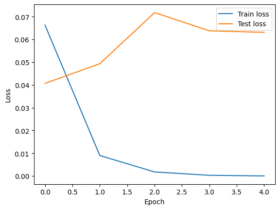
Let’s plot the loss of the model computed on the training and test sets.
Show code cell source
plt.plot(history['train_loss'], label='Train loss')
plt.plot(history['valid_loss'], label = 'Test loss')
plt.xlabel('Epoch')
plt.ylabel('Loss')
plt.legend()
plt.show()
We also evaluate the model on the test set and print the classification accuracy.
Show code cell source
ans = trainer.eval(model, test_loader)

print(f"Test accuracy: {ans['accuracy']:.2%}")
Test accuracy: 99.17%
Step 4: Fine-tuning with unfrozen backbone#
Finally, we unfreeze the last few layers of the convolutional backbone and train the model again with a very low learning rate.
WARNING: The code below may take a very long time to run.
model.unfreeze(3)

optimizer = optim.Adam(model.parameters(), lr=1e-5, amsgrad=True)

history = trainer.fit(model, train_loader, loss_fn, optimizer, epochs, test_loader)
===== Training on cuda device =====
Epoch  1/5: 100%|██████████| 293/293 [01:31<00:00,  3.19it/s, accuracy=0.9917, train_loss=0.0000, valid_loss=0.0801]
Epoch  2/5: 100%|██████████| 293/293 [01:28<00:00,  3.31it/s, accuracy=0.9923, train_loss=0.0000, valid_loss=0.0805]
Epoch  3/5: 100%|██████████| 293/293 [01:24<00:00,  3.49it/s, accuracy=0.9919, train_loss=0.0000, valid_loss=0.0812]
Epoch  4/5: 100%|██████████| 293/293 [01:23<00:00,  3.49it/s, accuracy=0.9917, train_loss=0.0000, valid_loss=0.0820]
Epoch  5/5: 100%|██████████| 293/293 [01:23<00:00,  3.49it/s, accuracy=0.9917, train_loss=0.0000, valid_loss=0.0828]
Let’s plot the loss of the model computed on the training and test sets.
Show code cell source
plt.figure(figsize=(10, 4))
plt.subplot(1,2,1)
plt.plot(history['train_loss'], label='Train loss')
plt.xlabel('Epoch')
plt.ylabel('Loss')
plt.title('Training loss')
plt.subplot(1,2,2)
plt.plot(history['valid_loss'], label = 'Test loss')
plt.xlabel('Epoch')
plt.ylabel('Loss')
plt.title('Test loss')
plt.show()
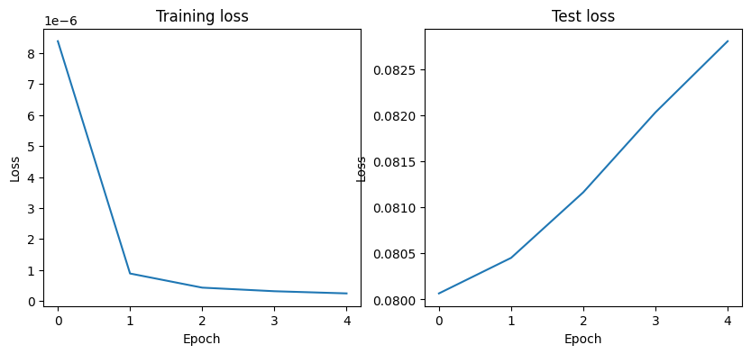
Note that the validation loss does not show any real improvement (in fact, it is deteriorating). You may wonder, how could accuracy improve if the loss isn’t decreasing? The answer is simple: what we display is an average of pointwise loss values, but what actually matters for accuracy is the distribution of the loss values, not their average, since accuracy is the result of a binary thresholding of the class probability predicted by the model. The model may still be improving even if this isn’t reflected in the average loss.
Now, let’s evaluate the fine-tuned model on the test set and print the classification accuracy.
Show code cell source
ans = trainer.eval(model, test_loader)

print(f"Test accuracy: {ans['accuracy']:.2%}")
Test accuracy: 99.17%
The accuracy of the fine-tuned model did not improve significantly compared to the model with the frozen backbone. This is because the task is relatively simple, and the performance of the model with the frozen backbone is already quite high. In practice, when the dataset is small and/or the task is complex, fine-tuning can significantly improve the performance of a pre-trained model.
Summary#
In this tutorial, we learned how to fine-tune a pre-trained model on a new dataset. We started by modifying the architecture of the pre-trained model to adapt it to the new task. We then prepared the dataset for the new task and trained the model with the convolutional backbone frozen. Finally, we fine-tuned the model by unfreezing some layers of the convolutional backbone and training it again with a very low learning rate. We also discussed the importance of keeping Batch Normalization layers frozen and in evaluation mode during fine-tuning to prevent them from updating their statistics and parameters.