Neural Networks#
Your goal is to develop a retrieval system that can search for images based on a predefined set of visual attributes. This system will leverage deep metric learning techniques to learn a shared embedding space where both images and their corresponding attributes can be compared effectively. The architecture consists of two separate neural networks:
A convolutional neural network (CNN) that generates embeddings from images.
A fully-connected neural network (MLP) that generates embeddings from attribute vectors.
Despite processing different types of data, both networks are designed to produce outputs in the same embedding space, allowing for direct comparison between images and attributes.
Architecture#
The figure below illustrates the overall architecture for processing a triplet, which includes an image, a positive attribute vector, and a negative attribute vector. In this setup, the image network (highlighted in blue) processes the image, while the attribute network (highlighted in yellow) processes both positive and negative attribute vectors in a Siamese-like configuration. The networks map their inputs into a shared embedding space, enabling the calculation of similarity scores between images and attributes.
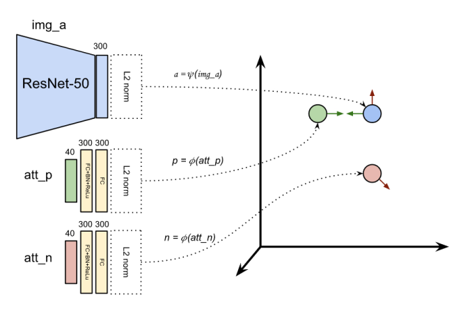
Network details#
The dimensionality of the embedding space is chosen based on the complexity of the relationships you wish to capture. While typical dimensions range from 100 to 500, this project employs a 300-dimensional space to balance expressiveness with computational efficiency.
A convolutional neural network is used to generate image embeddings. The network leverages a pre-trained backbone (such as MobileNet or ResNet-50) for robust feature extraction, followed by a custom head that maps these features into the 300-dimensional embedding space. The output is normalized to ensure that all image embeddings have unit length, simplifying subsequent similarity computations.
A fully connected network is used to generate embeddings for attributes. This network comprises two linear layers (each with 300 dimensions) interleaved with batch normalization and ReLU activation to introduce non-linearity and promote training stability. Similar to the image embeddings, the output is normalized to produce unit-length vectors, ensuring compatibility in the shared embedding space.
Pretraining#
The image network comprises a convolutional backbone and a fully-connected head. To facilitate training, the backbone can be taken from a pre-trained model, such as MobileNet or ResNet-50, to leverage the robust feature extraction capabilities of these architectures. In contrast, the image network’s head and the attribute network are randomly initialized to enable learning of the shared embedding space.
Recommendation
Begin with a feature extraction strategy to rapidly establish a functional system with stable and robust representations. Once you have a reliable baseline, explore fine-tuning to further enhance the model’s performance on your specific dataset.
Feature extraction#
In the feature extraction strategy, the backbone of the image network is kept frozen, while the embedding head is trained from scratch. When dealing with high-dimensional data like images, however, training a network directly on raw pixels can be computationally intensive, even when the backbone is pre-trained and frozen. To mitigate this issue, you can precompute the backbone output for all images in the dataset and store these features for subsequent training. This approach significantly reduces the computational burden, as the backbone only needs to be run once per image, rather than once per training iteration.
Practical details#
The Weak Supervision tutorial provides a detailed implementation for extracting image features using a pre-trained backbone. In summary, the process involves the following steps.
Create a standard CNN with pre-trained weights.
Create the dataset using the model transform as preprocessing.
Loop through the dataset with a dataloader.
For each batch of images and attributes:
Extract the image features using the pre-trained model.
Store the image features and attributes in two separate lists.
At the end of the loop, stack the image features and attributes into tensors.
Save the tensors to disk for future training.
Note
A PyTorch tensor can be saved to disk using the torch.save function. The saved tensor can be loaded using the torch.load function.
Tensor dataset#
The image features and attributes can be combined into a dataset using the TensorDataset class. The following code snippet demonstrates how to do this.
import torch
from torch.utils.data import TensorDataset

# Load the saved tensors
features   = torch.load('features.pt')
attributes = torch.load('attributes.pt')

# Create a dataset from the tensors
dataset = TensorDataset(features, attributes)

# Example of accessing the first element in the dataset
feat0, attr0 = dataset[0]
Alternatively, you can define a custom dataset that loads the tensors and returns them as needed.
import os
import torch
from torch.utils.data import Dataset

class CustomDataset(Dataset):

    def __init__(self, root_dir):
        self.features = torch.load(os.path.join(root_dir, 'features.pt'))
        self.attributes = torch.load(os.path.join(root_dir, 'attributes.pt'))

    def __len__(self):
        return len(self.features)

    def __getitem__(self, idx):
        return self.features[idx], self.attributes[idx]
Training#
Once the image features and attributes are precomputed and stored, you can train the networks using the custom dataset created in the previous step. You can reuse the training loop from the tutorials by providing the appropriate adapter. In this case, you need to group the two networks into a single model to comply with the expected interface. The general approach is similar to the Weak Supervision tutorial.
class EmbeddingNetworks(torch.nn.Module):

    def __init__(self):
        super().__init__()
        self.image_net = ...     # torch.nn.Module
        self.attribute_net = ... # torch.nn.Module
def my_adapter(model: EmbeddingNetworks,
               batch: tuple[torch.Tensor, torch.Tensor],
               loss_fn: torch.nn.Module) -> float:

    # Unpack the batch
    features, attributes = batch

    # Forward pass
    ...

    # Loss computation
    loss = ...

    return loss