Data Preparation#
Previously, the dataset was filtered so that each image contained at most one instance of the target class. Now you will keep all images, with some containing one or more objects of the chosen class, and others containing none. The Pascal VOC Detection dataset already provides the necessary annotations. However, these annotations must be converted into a format suitable for grid-based dense prediction.
Pretrained model#
A key design choice in multi-object localization is the selection of the convolutional backbone. The backbone not only extracts features from the input image but also determines the spatial resolution of the final feature map. This resolution is crucial, as it defines the S×S grid of cells used for bounding box prediction. As a concrete example, we will examine two representative pretrained backbones available in Torchvision, MobileNet and SSDLite, highlighting how their architectures influence the grid resolution.
Mobile Net#
MobileNetV3 is an image classification model trained on ImageNet dataset. Its architecture progressively reduces the spatial dimensions of the input image, reaching a reduction factor (stride) of 32. For a 224×224 input image, MobileNetV3 produces a final feature map of size 7×7.
Show code cell source
import torch
from torchvision.models import mobilenet_v3_large, MobileNet_V3_Large_Weights

weights = MobileNet_V3_Large_Weights.DEFAULT
model = mobilenet_v3_large(weights=weights)
model.eval()

images = torch.randn(1, 3, 224, 224)  # batch size, channels, height, width

with torch.inference_mode():
    features = model.features(images)

print(f"Input  size: {tuple(images.shape)}")
print(f"Output size: {tuple(features.shape)}")
Input  size: (1, 3, 224, 224)
Output size: (1, 960, 7, 7)
SSD Lite#
SSDLite320 is an object detection model trained on COCO dataset. Its architecture builds upon MobileNetV3 backbone, incorporating additional layers to produce feature maps at different resolutions. For a 320×320 input image, SSDLite320 generates feature maps of sizes 20×20, 10×10, 5×5, 3×3, 2×2, and 1×1, corresponding to reduction factors (strides) of 16, 32, 64, 106.666…, 160, and 320, respectively.
Show code cell source
import torch
from torchvision.models.detection import ssdlite320_mobilenet_v3_large, SSDLite320_MobileNet_V3_Large_Weights

weights = SSDLite320_MobileNet_V3_Large_Weights.DEFAULT
model = ssdlite320_mobilenet_v3_large(weights=weights)
model.eval()

images = torch.randn(1, 3, 320, 320)  # batch size, channels, height, width

with torch.inference_mode():
    features = model.backbone(images)

print(f"Input  size: {tuple(images.shape)}")
print(f"Output size:", *[tuple(features[key].shape) for key in features], sep="\n  ")
Input  size: (1, 3, 320, 320)
Output size:
  (1, 672, 20, 20)
  (1, 480, 10, 10)
  (1, 512, 5, 5)
  (1, 256, 3, 3)
  (1, 256, 2, 2)
  (1, 128, 1, 1)
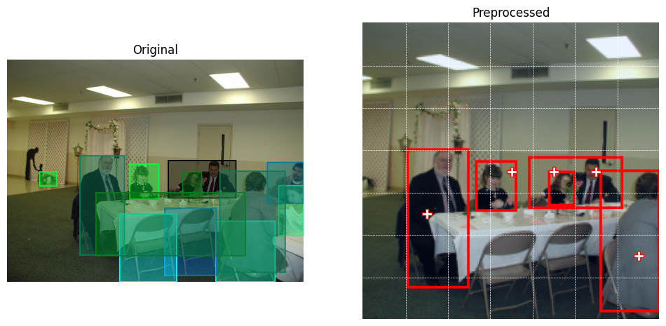
Preprocessing#
Prior to training, each sample in the dataset is preprocessed using the following pipeline.
Transformations
The image is resized and cropped to match the input size expected by the chosen backbone.
Pixel values are normalized using the same statistics as those used during backbone pretraining.
Bounding box coordinates are adjusted to maintain alignment with the transformed image.
Degenerate boxes arising from these transformations are filtered out (e.g., boxes that fall completely outside the image boundaries after cropping).
Label assignment
The annotations of each image are converted into tensors matching the grid size of the chosen backbone. Every grid cell is assigned a label consisting of an objectness indicator and bounding box coordinates. The objectness indicator is a binary value set to 1 if the cell contains an object and 0 otherwise. If a cell contains an object, its bounding box coordinates are assigned to the label. Otherwise, the label is assigned dummy coordinates (e.g., all zeros).
Optionally, the bounding box coordinates can be normalized by the image size.
After preprocessing, each image is paired with a tensor of shape (1+4) x S × S. The first channel contains objectness indicators, and the remaining four channels contain bounding box coordinates. This structure allows the model’s detection head to process all grid cells simultaneously during training.
Note
A grid cell is considered to contain an object if the bounding box center falls within the cell’s boundaries. Nearby cells can also be assigned the same object to improve detection robustness.
Conflict Resolution
It is possible for multiple objects to fall into the same cell. In such cases, a strategy must be employed to decide which object to assign to the cell. Common strategies include selecting the object with the smallest area, the largest area, or the one closest to the cell center.
Validation and Debugging#
It is important to validate the preprocessing pipeline to ensure that images and target tensors are aligned correctly. Common checks include the following.
Visualizing bounding boxes. Overlay the preprocessed bounding boxes on the corresponding preprocessed image to confirm that object alignment is preserved. (You will need to denormalize coordinates back to pixel values.)
Grid assignment sanity check. For a few images, verify that object centers are assigned to the expected grid cells.
Target tensor inspection. Print or visualize slices of the target tensor to confirm that objectness indicators match the annotations.
These debugging steps are crucial: errors in preprocessing (e.g., incorrect scaling, misaligned boxes, or wrong grid assignments) often manifest later as poor training performance. By validating early, you can isolate problems in the data pipeline before introducing model complexity.