Training#
This section describes the design of the single-object localization model, the loss function used for training, and the overall training procedure.
Model architecture#
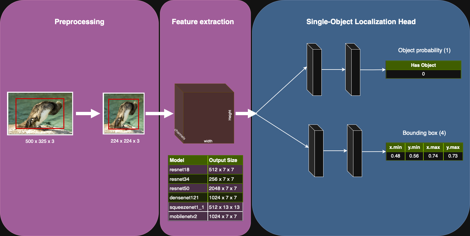
The model builds on precomputed features extracted using MobileNetV3 (see previous section). These feature vectors serve as the input to a small custom neural network, often referred to as the single-object localization head. The head is divided into two branches.
Classification branch. It predicts whether the target object class is present in the image.
This branch consists of two fully connected layers with a ReLU activation in between.
The final output is a single scalar that represents the “logit” score for binary classification.
Regression branch. It predicts the bounding box coordinates \((x_{\min}, y_{\min}, x_{\max}, y_{\max})\) normalized with respect to the image size.
This branch also uses two fully connected layers separated by ReLU activation.
Batch Normalization can be applied after the first layer to stabilize training.
The final layer uses a sigmoid activation, which bounds the output between 0 and 1.
The two branches share the same input features but operate independently, allowing the network to learn classification and localization tasks in parallel. The combined output of the model is a tuple containing the classification score (scalar) and the bounding box coordinates (vector of length 4).
Loss function#
Training the model requires optimizing both the classification of object presence and the regression of bounding box coordinates. These two objectives are handled by distinct loss functions.
Binary Cross-Entropy (BCE) loss is applied to the classification branch, comparing the predicted logit score with the ground-truth label (0 or 1).
Smooth L1 loss is applied to the regression branch, comparing the predicted normalized coordinates with the ground-truth bounding box.
The total loss is defined as the sum of these two components:
where \(\lambda\) controls the relative importance of classification vs. localization. In practice, \(\lambda = 1\) is often a good starting point.
Note
Since bounding boxes are only defined when the object is present, the regression loss must be computed only for positive examples. For negative examples (label = 0), no bounding box exists, so only the classification loss contributes to training. This prevents the model from being penalized for incorrect bounding box predictions when the object is absent.
Training Procedure#
The training loop follows the standard supervised learning recipe in PyTorch. You can reuse the training loop from the tutorials by providing the appropriate train_step() function. As a reminder, this function should perform the following steps:
Forward pass: Pass the features through the model to obtain predictions for both classification and bounding box regression.
Loss computation: Evaluate the loss using the predicted logit scores and bounding boxes, as well as the ground-truth labels and bounding boxes.
Backward pass: Compute gradients and update the parameters of the model using the optimizer.
def train_step(model: LocalizationNet,
               batch: tuple[Tensor, Tensor, Tensor],
               loss_fn: 'LocalizationLoss',
               optimizer: torch.optim.Optimizer,
               device: torch.device) -> float:

    feats, labels, bboxes = batch
    feats, labels, bboxes = feats.to(device), labels.to(device), bboxes.to(device)

    ... # Your code here

    return loss.item()
Learning curve#
During training, the total loss should decrease steadily over epochs. The plot below shows a typical training curve obtained with a correct implementation.
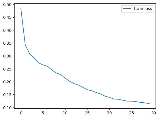
If your training curve does not behave like this (for example, if the loss stays flat or oscillates wildly), it is a strong indication that there is an error in the pipeline. Common issues include:
Mismatch between preprocessing of images and bounding boxes.
Incorrect application of sigmoid activations or loss functions.
Forgetting to normalize bounding box coordinates between 0 and 1.
Incorrect handling of labels (e.g., not using 0/1 for binary classification).
Always verify your preprocessing and double-check your loss computation if the training curve does not descend as expected.
Negative sampling#
In single-object localization, the dataset contains many more images without the target object (negative examples) than images with the object (positive examples). If the model is trained on the raw dataset distribution, it can become biased toward predicting “no object,” since that minimizes the classification loss on most training examples. To ensure balanced training, it is important to control how many negative examples are included in each training epoch.
The imbalance is handled using a custom sampler, connected to the PyTorch DataLoader to control which examples are drawn each epoch. The sampler ensures that all positive examples are included in every epoch, and then adds a controlled number of negative examples, selected randomly. The ratio between negatives and positives is adjustable through a parameter. At the start of each epoch, the sampler shuffles the selected positive and negative indices so that the model does not see the same ordering twice. This prevents overfitting and ensures a fair mix of examples during training.
The code below implements a balanced sampler that can be used with the DataLoader. It takes as input the list of labels (0 or 1) for all examples in the dataset, and a negative_ratio parameter that controls how many negative examples to include per positive example.
import torch
import numpy as np


class BalancedSampler(torch.utils.data.Sampler):

    def __init__(self, labels: list[int], negative_ratio=1.0):
        """
        Args:
            labels: Binary array or list, where 1=positive, 0=negative.
            negative_ratio (float): Fraction of negatives to sample per epoch.
        """
        labels = np.array(labels)
        self.positive_indices = np.where(labels == 1)[0]
        self.negative_indices = np.where(labels == 0)[0]
        self.pos = len(self.positive_indices)
        self.neg = int(round(self.pos * negative_ratio))
        assert self.pos > 0, "The number of positives is zero."
        assert self.neg > 0, "The number of negatives is zero."
        if self.neg > len(self.negative_indices):
            self.neg = len(self.negative_indices)
            print(f"Warning: Only {len(self.negative_indices)} negatives are available. Adjusting ratio to {self.neg / self.pos:.2f}.")

    def __iter__(self):
        indices = np.empty(self.pos + self.neg, dtype=np.int64)
        indices[:self.pos] = self.positive_indices
        indices[self.pos:] = np.random.choice(self.negative_indices, size=self.neg, replace=False)
        np.random.shuffle(indices)
        return iter(indices.tolist())

    def __len__(self):
        return self.pos + self.neg