
1. Supervised Learning#
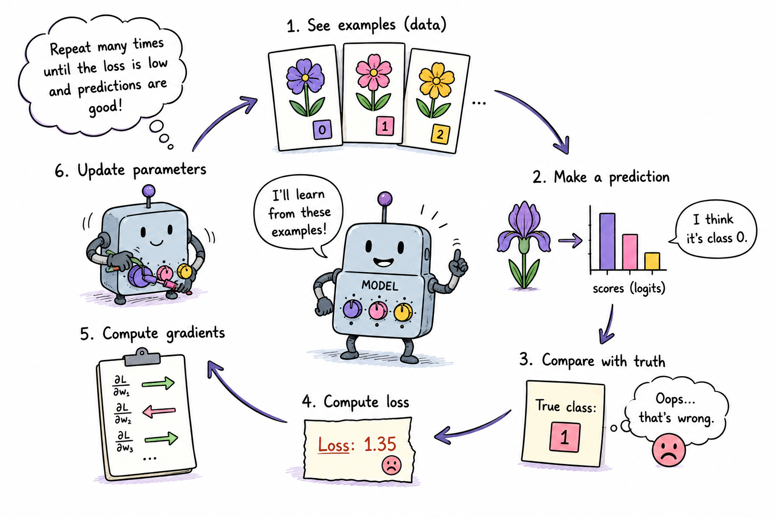
Suppose we want to build a program that can identify a species of flower from four measurements: the length and width of its sepals and petals. We have already collected measurements from many flowers, and a botanist has identified the species of each one. For one flower, the data might look like this.
sepal length: 5.1 cm
sepal width:  3.5 cm
petal length: 1.4 cm
petal width:  0.2 cm
species:      setosa
Our goal is to build a program that receives the four measurements of a new flower and predicts its species. A traditional program would need explicit rules written by a programmer. But writing reliable rules becomes difficult when several measurements interact or when different species overlap. Instead, we will build a model whose behaviour is determined by adjustable numbers. The model will begin with poor values for those numbers and improve them by examining labelled examples. This process is called learning.
1. Dataset#
Each flower is one example. The four measurements are its features, and the known species is its target. We can represent one example as a vector.
The target can be represented by an integer.
0 → setosa
1 → versicolor
2 → virginica
The integer is only a code. It does not imply that virginica is “larger” than versicolor or that the distance between classes 0 and 1 has a numerical meaning.
When several examples are collected into one array, each row represents one flower and each column represents one feature.
This array has shape (3, 4). The first dimension counts examples; the second dimension counts features. The corresponding targets might be a vector of integers.
The target array has shape (3,) because there is one target for each example. This relationship between shapes is not an implementation detail. It is part of the definition of the learning problem. If X contains 150 examples, y must contain 150 targets.
Quiz
Suppose X.shape is (200, 4).
What does
X[12]represent?What does
X[:, 2]represent?
Answer
`X[12]` is one example containing four features. `X[:, 2]` is the third feature collected from all 200 examples.2. Model and parameters#
A model receives an input and produces an output. In mathematical notation, we can represent the model as a function that maps an input \(x\) to an output \(z\), and depends on some parameters \(\theta\).
The input changes from one flower to another. The parameters belong to the model and are the same for every flower. The model’s behaviour is determined by the values of its parameters.
The simplest model is a linear function. It combines the input features with the model’s parameters using a weighted sum.
This model contains two sets of parameters: a weight matrix \(W\) and a bias vector \(b\). They form the set of trainable parameters \(\theta = (W, b)\).
For our flower problem, the input contains four features and the model must produce three class scores. The shapes of the different arrays are therefore as follows.
x: (4,)
W: (4, 3)
b: (3,)
z: (3,)
Multiplying the input by the weight matrix combines the four measurements into three output values. Adding the bias adjusts each output independently.
For a batch of flowers, the same computation produces a matrix of outputs.
If X has shape (150, 4), then Z has shape (150, 3). Each row contains three scores for one flower.
In NumPy or PyTorch, the forward computation is only one line.
logits = x @ weights + bias
The simplicity of the code can hide an important fact: the model is applying the same learned rule to every example in the batch.
3. Prediction scores#
The three output values are called logits. A possible output might be like this.
logits = [2.3, -0.4, 0.7]
The first value is the score for class 0, the second for class 1, and the third for class 2. The model’s prediction is the class with the largest score. For the logits above, the predicted class is 0.
prediction = logits.argmax()
A logit is not a probability. It can be positive or negative, and the logits do not need to add up to one. They are unrestricted scores that express the model’s relative preference for each class. This separation is useful:
the model outputs class scores,
the prediction rule selects the class with the largest score.
During training, we need more than the final class decision. We need to know whether the correct class received a slightly lower score or a dramatically lower score than the alternatives. The complete set of logits preserves that information. Consider two predictions for a flower whose correct class is 0.
logits_A = [2.1, 2.0, 1.9]
logits_B = [8.0, 0.2, -1.0]
Both predict class 0. But the model is much more decisive in case B. A training objective can distinguish between these two cases even though the final predicted class is the same.
4. Loss function#
At the beginning of training, the parameters are not useful. The model may assign high scores to the wrong classes or nearly identical scores to every class. To improve the model, we need a numerical measure of how poor its outputs are. This measure is called the loss function.
For multiclass classification, we commonly use cross-entropy loss. It compares the logits with the correct target and produces one number. A low loss means that the model gives a relatively high score to the correct class. A high loss means that the correct class receives too little support compared with the alternatives.
Mathematically, we can express the loss function as:
where \(Z\) contains the model’s logits, \(y\) contains the correct classes, and \(L\) is the loss value. Even when the model processes many examples and produces many logits, the final loss is usually reduced to one number. This gives training a single objective to improve.
The loss is not the same as accuracy. Accuracy measures how many predictions were correct. The loss measures how well the model supported the correct classes relative to the alternatives. A model can become better according to the loss before its accuracy changes. For example, it may increase the score of the correct class without yet making it the largest score.
Quiz
Suppose the correct class is 2. Which output does have the lower loss?
A: [3.0, 1.0, 2.5]
B: [0.1, 0.3, 4.2]
Answer
Output B should have the lower loss because the correct class receives the largest score by a wide margin.5. Gradients#
Once we have calculated the loss, we know whether the current parameters produced good or poor outputs. But the loss alone does not tell us which parameters should change. The model may contain many weights. Increasing one weight might lower the loss, while increasing another might raise it. Some parameters may have a large effect; others may currently have almost no effect.
For each parameter, we need to know how the loss would change if we adjusted that parameter. The answer is given by the parameter’s gradient. For a single parameter \(\theta_i\), the partial derivative \(\frac{\partial L}{\partial \theta_i}\) describes how the loss responds to a small change in that parameter. A positive gradient means that increasing the parameter would increase the loss locally. A negative gradient means that increasing the parameter would decrease the loss locally. The magnitude indicates how sensitive the loss is to that parameter near its current value. A model with many parameters has a gradient value for every parameter. Together, these values form the gradient of the loss.
Calculating all those derivatives manually would quickly become impractical. PyTorch records the operations used to compute the logits and the loss. At the user’s request, PyTorch can replay those operations in reverse order and calculates the gradient of the loss with respect to every trainable parameter involved in the computation. This process is called automatic differentiation.
6. Optimization#
The gradient points in the direction in which the loss increases most rapidly. To reduce the loss, we move the parameters in the opposite direction. For one parameter, the update is a simple subtraction.
The symbol \(\eta\) represents the learning rate and determines the size of the update. A very small learning rate produces tiny changes to the parameters. A well-chosen learning rate can reduce the loss steadily, but if it is too large, it can overshoot useful parameter values and make training unstable.
In code, a manual update might look like this.
with torch.no_grad():
    weights -= learning_rate * weights.grad
    bias -= learning_rate * bias.grad
The update is placed inside torch.no_grad() because it is an action performed by the training procedure. We do not want PyTorch to treat the update itself as part of the model’s differentiable computation. After the update, the stored gradients must be cleared to avoid accumulating them across multiple training steps.
7. Training loop#
One parameter update is rarely enough. Training repeats the same sequence many times: compute logits, compute the loss, calculate gradients, update the parameters, clear the gradients. Repeating these steps gradually changes the function represented by the model. A minimal training loop looks like this.
for step in range(number_of_steps):

    logits = x @ weights + bias

    loss = torch.nn.functional.cross_entropy(logits, targets)

    loss.backward()

    with torch.no_grad():
        weights -= learning_rate * weights.grad
        bias -= learning_rate * bias.grad

    weights.grad.zero_()
    bias.grad.zero_()
After training, the model still contains only numbers: the entries of \(W\) and \(b\). Those numbers encode relationships between the input features and the output classes. A positive weight may cause a particular measurement to increase one class score. A negative weight may cause it to decrease another.
The model has not stored explicit rule such as “long petals usually indicate virginica”. Instead, that relationship is distributed across the parameters and expressed through a linear computation. This distinction matters. Training does not insert facts into the model one at a time. It adjusts parameters so that the model’s outputs become more useful across the examples it sees.
A model can also learn misleading relationships. If every flower of one species was photographed or measured under different conditions, the model might exploit those accidental differences. A decreasing training loss proves only that the model is becoming better at the objective on the training data. It does not prove that the model has learned a reliable rule. That is why we later evaluate the model on examples that were not used to update its parameters.
8. Evaluation#
A model is useful only if it can make good predictions on examples it has not seen before. To test this, we set aside a portion of the dataset for evaluation. The model does not see these examples during training. After training, we measure its accuracy on the evaluation set. A high accuracy indicates that the model has learned a relationship that generalizes beyond the training examples.
Training and evaluation answer different questions. During training, we ask whether the parameters can be adjusted to reduce the loss on the training examples. During evaluation, we ask whether the learned model can make useful predictions on examples it has not seen before. A model that performs well on training data but poorly on new data has overfit. It has adapted too closely to the training examples and has not learned a relationship that transfers reliably.
9. Conclusion#
The learning process can be summarized as a cycle of repeated steps.
Each step begins with a batch of examples.
The model transforms the input features into logits.
The loss compares the logits with the targets.
Automatic differentiation calculates parameter gradients.
The training procedure updates the parameters.
Repeated updates can reduce the loss.
Evaluation tests whether the learned model works on unseen examples.
This structure is not limited to linear classifiers. A neural network uses a more complex model. A retrieval system produces embeddings rather than class logits. An object detector predicts coordinates. But the underlying learning cycle remains recognizable.
Final quiz#
A model processes two different flowers. Which values change between the two forward passes: the input features, the parameters, or both?
Why does a three-class model produce three logits instead of directly producing one class number?
Can the loss decrease while accuracy remains unchanged?
What does a parameter gradient describe?
Why do we subtract the gradient?
Why is a low training loss not enough to conclude that the model is useful?