
3. Training Workflow#
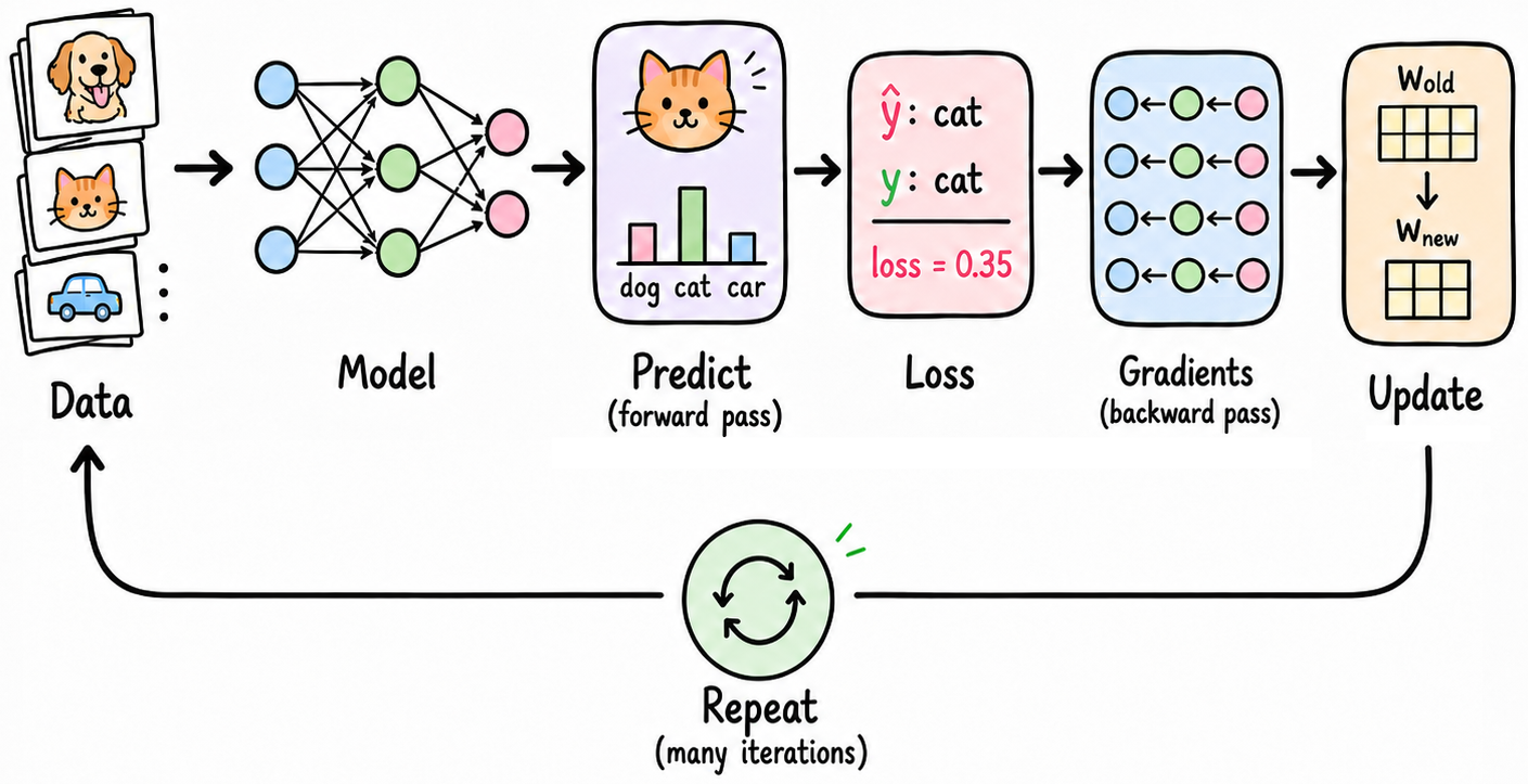
Training a neural network is a cycle. The model receives input data, produces predictions, compares them against the correct answers, and uses the resulting error to adjust its parameters so that future predictions improve. While this cycle is conceptually simple, applying it in practice requires careful organization. Real datasets cannot always be processed all at once. Instead, they are divided into smaller groups, and the model is updated repeatedly as it moves through these groups. At the same time, the model must be continuously evaluated to monitor its progress on long training runs.
In this lesson, we will build a complete training workflow that can load examples, organize them into batches, update the model repeatedly, evaluate it on separate data, record its progress, and retain the best version observed during training. The model itself is no longer the main subject. We will continue using a small neural network, but our attention will shift to the system around it.
1. Data organization#
Large datasets, such as ImageNet, contain millions of images. They usually do not fit in memory at once. Even if they do, processing all examples in one operation can be slow and inefficient. The model also needs memory for intermediate activations. During training, PyTorch retains information from the forward pass so that it can calculate gradients during backpropagation. Processing more examples at once therefore increases memory use throughout the network, not only at the input.
Instead of processing the complete dataset in one operation, we divide it into smaller groups called batches. Each batch produces one loss, one backward pass, and one parameter update. The training process then loops over many batch updates, each using a different subset of training data. The model sees the complete dataset over time, but only a limited number of examples are active in memory during any one update.
Batches serve both computational and statistical purposes. In addition to reducing memory requirements, they introduce variation into the gradient estimates. Each batch produces a slightly different estimate of the gradient, so the optimization steps are not identical to the ones produced by training on the complete dataset. This variation can sometimes help the model find solutions that generalize better to unseen data.
Terminology
A sample is one example from a dataset.
A batch is a collection of samples processed together.
An iteration (training step) is one parameter update performed using one batch.
An epoch is one complete pass through the training dataset.
Example
Suppose a dataset contains 1,000 examples and the batch size is 100. One epoch contains ten batches and therefore ten parameter updates. If the batch size is 64, the dataset does not divide evenly. The epoch contains 16 batches, with the first 15 containing 64 examples, and the final batch containing the remaining 40. This smaller final batch is important when we calculate averages for one epoch. We cannot always treat every batch as if it represented the same number of examples.
Quiz
A dataset contains 12,000 examples and uses batches of 200. How many parameter updates occur during one epoch?
Answer
There are (12,000 / 200 = 60) batches, so the model receives 60 parameter updates per epoch.Representing a dataset#
A model does not need to know how examples are stored. It only needs to receive tensors with the expected shapes and dtypes. The responsibility for locating and returning examples belongs to a dataset. In PyTorch, a dataset behaves like a collection and provides two basic operations.
__len__returns the number of examples in the dataset.__getitem__returns the example associated with a particular index (e.g., an input-target tuple).
A dataset is commonly implemented as a subclass of torch.utils.data.Dataset. This approach becomes useful when examples require special loading or preprocessing. Such a class normally implements the two basic operations mentioned above, but it can also support other functionality, such as the ability to apply transformations to the retrieved examples.
class ExampleDataset(torch.utils.data.Dataset):

    def __len__(self):
        return ... # number of examples

    def __getitem__(self, index):
        features = ...
        target = ...
        return features, target
For data already stored in tensors, PyTorch provides TensorDataset to ensure a consistent interface.
Quiz
Does a Dataset decide how many examples belong in one training batch?
Answer
No. The dataset only defines access to individual examples.Iterating over batches#
A DataLoader retrieves examples from a dataset and groups them into batches. Iterating over a data loader gives one batch at a time, until all examples have been exhausted, after which the iteration stops.
from torch.utils.data import DataLoader

training_loader = DataLoader(training_dataset, batch_size=64, shuffle=True)

for features, targets in training_loader:
    print(features.shape)
    print(targets.shape)
    break
Data loaders rely on a collate function to combine individual examples into a batch. The default collate function stacks tensors along a new first dimension, while preserving the general structure of the individual examples. If the dataset returns tuples of two tensors with shapes (3,) and (), the resulting batch is a tuple of two tensors with shapes (batch_size, 3) and (batch_size,).
Note
Datasets and loaders are separate because they solve different problems in the machine learning workflow. The dataset is responsible for providing individual examples, and each new task may require a different dataset. The loader is responsible for batching and shuffling, two operations that are shared across tasks. The learning algorithm relies on a loader to produce batches of training data. It does not need to know where the data comes from or how they are organized. This separation allows the same training loop to work seamlessly with different datasets.
Shuffling#
Training loaders normally use shuffle=True. This causes the order of the training examples to change randomly before they are grouped into batches. Shuffling is especially important when the original dataset is ordered by class, time, source, or another meaningful property. Without shuffling, early batches might contain mostly one class while later batches contain another. The gradients would then reflect the ordering of the dataset rather than a representative mixture of examples.
Loaders used for evaluation and testing normally do not shuffle. The evaluation phase does not update the model, so the order of examples does not matter. A stable order also makes it easier to associate predictions with particular examples during error analysis.
Quiz
Would shuffling the validation loader change the final validation accuracy?
Answer
No. Accuracy depends on the predictions and targets, not on the order in which examples are processed. A stable validation order is nevertheless useful for reproducibility and error analysis.Batch size#
Batch size affects both computation and learning. Larger batches make better use of parallel hardware and produce gradients based on more examples, but they require more memory and create fewer updates per epoch. Smaller batches require less memory and produce more frequent updates, but their gradients vary more from one batch to another. There is no universally correct batch size. It is a training choice whose effects depend on the model, data, hardware, and optimizer. For now, the important point is that batch size changes how the same dataset is divided into update steps.
2. Training#
Training a model requires repeated updates to its parameters. Each update is based on a batch of examples, and the model must see all examples multiple times to learn effectively. This requires two levels of repetition: the outer loop counts complete passes through the dataset, while the inner loop processes the individual batches in the current epoch. The snippet below shows the basic structure of a training loop.
for epoch in range(number_of_epochs):

    for features, targets in training_loader:
        ...
Training step#
The operations inside the inner loop are the same ones used previously. The difference is that they now operate on a batch rather than the complete training set. The batch changes at every iteration, but the model parameters persist. Each update therefore reflects information from a different subset of training examples.
def train_batch(model, batch, loss_fn, optimizer, device):

    features, targets = batch
    features = features.to(device)
    targets = targets.to(device)

    outputs = model(features)
    loss = loss_fn(outputs, targets)

    optimizer.zero_grad()
    loss.backward()
    optimizer.step()

    return loss.item()
The batch is moved to device before the forward pass. This must be the same device on which the model is located. Keeping device placement explicit inside the batch-processing function makes the workflow compatible with both CPU and GPU execution without changing the rest of the training logic.
Batch loss#
A loss function is usually defined as the average loss over the examples on which it is evaluated. This ensures that the loss is independent of the batch size. If a batch contains \(B\) examples with individual losses \(\ell_1,\ell_2,\ldots,\ell_B\), the returned loss is
The optimizer updates the parameters immediately after each batch is processed. The next batch is hence processed by a slightly different model. This means that the loss reported by one batch describes the model’s performance on that particular group of examples at that particular moment in training.
Epoch loss#
A single batch gives a partial view of performance. To describe the full training set, we need to aggregate information across every batch. Since the final batch may contain fewer examples than the others, we cannot simply average the batch losses to obtain an unbiased estimate. Instead, we need to weight each batch by its number of examples. The mean loss for one epoch is therefore
where \(B\) is the number of batches, \(B_b\) is the number of examples in batch \(b\), \(L_b\) is the loss for batch \(b\), and \(N\) is the total number of examples in the dataset. This calculation ensures that every example contributes equally to the epoch loss, regardless of which batch it was processed in.
Note
Accuracy and other metrics can be accumulated in a similar way.
Quiz
Why is the unweighted mean of batch losses unreliable when the final batch is smaller?
Answer
Each batch loss is already a mean. Averaging those means gives every batch equal importance, even when one batch represents fewer examples. Weighting by batch size gives every example equal importance.Training epoch#
A complete training epoch can be organized as follows. For each batch, we perform a training step and compute the batch loss. Multiplying by batch_size recovers the total contribution from that batch. After processing all batches, we divide the total loss by the total number of examples to obtain the epoch loss.
def train_epoch(model, loader, loss_fn, optimizer, device):
    model.train()

    total_loss = 0.0
    total_examples = 0

    for features, targets in loader:
        loss = train_batch(model, (features, targets), loss_fn, optimizer, device)

        batch_size = targets.shape[0]
        total_loss += loss * batch_size
        total_examples += batch_size

    return total_loss / total_examples
Calling model.train() places the model in training mode. This is important for layers such as dropout and batch normalization that behave differently during training and evaluation. Switching to training mode ensures that the model behaves consistently during learning, regardless of whether it contains such layers.
3. Evaluation#
Training updates the model repeatedly, but we also need to monitor its performance on separate data. The training and evaluation phases share some computations, but their purposes are different enough to justify separate functions. A minimal evaluation function, only computing the loss, can be organized as follows.
def evaluate(model, loader, loss_fn, device):
    model.eval()

    total_loss = 0.0
    total_examples = 0

    with torch.inference_mode():
        for features, targets in loader:

            features = features.to(device)
            targets = targets.to(device)

            outputs = model(features)
            loss = loss_fn(outputs, targets)

            batch_size = targets.shape[0]
            total_loss += loss.item() * batch_size
            total_examples += batch_size

    return total_loss / total_examples
Calling model.eval() places the model in evaluation mode. Some layer types behave differently during training and evaluation. Dropout and batch normalization are important examples that we will study later. It should be called systematically before evaluation to ensure that the evaluation function behaves correctly with any architecture. Calling model.train() restores training mode again.
During evaluation, the model parameters are not updated. Recording the operations needed for gradient calculation would waste memory and computation. The python line with torch.inference_mode(): creates a context where PyTorch does not build the gradient-tracking graph for the operations inside it.
Important
A correct evaluation procedure must use two PyTorch mechanisms.
model.eval()to switch layers into evaluation mode.torch.inference_mode()to disable gradient recording.
Quiz
Which statement is correct?
model.eval()prevents the optimizer from updating parameters.torch.inference_mode()changes dropout into evaluation behaviour.model.eval()andtorch.inference_mode()have different responsibilities.Neither is necessary if the validation set is small.
Answer
`model.eval()` changes the operating mode of layers whose behaviour differs between training and evaluation. `torch.inference_mode()` disables gradient recording. They are complementary rather than interchangeable.Monitoring#
One epoch gives a single snapshot of the model’s performance. To understand how the model changes over time, we can record the training and validation losses for every epoch. This information can be used for plotting learning curves, detecting early stopping, or selecting the best model observed during training. The following snippet shows how to record the losses for every epoch.
history = {
    "train_loss": [],
    "valid_loss": [],
}

for epoch in range(number_of_epochs):

    train_loss = train_epoch(model, training_loader, loss_fn, optimizer, device)

    valid_loss = evaluate(model, validation_loader, loss_fn, device)

    history["train_loss"].append(train_loss)
    history["valid_loss"].append(valid_loss)
Plotting these values reveals how the model changes over time. A single final metric cannot show whether training was stable, whether progress stopped early, or whether validation performance deteriorated after initially improving. The interpretation of those patterns will be developed in the next lesson. For now, the important point is that a reliable workflow records enough information to make such analysis possible.
Note
Training batches within one epoch are processed by a slightly different model. The first batch is processed before any updates from that epoch, while the last batch is processed after many updates. The training loss for an epoch is therefore a summary of a changing model rather than a measurement taken at one fixed parameter state. That is acceptable for monitoring training, but it should be understood clearly. This is different from evaluation, where the model is not updated and performance metrics are measured at one fixed parameter state.
Checkpointing#
The best model observed during training may not be the one from the final epoch. This is due to validation performance fluctuating over the course of training. To preserve the best model, we can save a checkpoint whenever validation performance improves. A checkpoint is a saved model state, usually accompanied by information such as the epoch, optimizer state, and validation metric.
import copy

best_valid_loss = float("inf")
best_state = None

for epoch in range(number_of_epochs):

    _ = train_epoch(model, training_loader, loss_fn, optimizer, device)

    valid_loss = evaluate(model, validation_loader, loss_fn, device)

    if valid_loss < best_valid_loss:
        best_valid_loss = valid_loss
        best_state = copy.deepcopy(model.state_dict())
At the end of training, the selected state is restored to the model with load_state_dict. The workflow therefore retains the best model observed during training, not necessarily the one from the final epoch.
Quiz
A network reaches its lowest validation loss at epoch 42. Training continues to epoch 100, where the training loss is lower but validation loss is higher. Which checkpoint should be selected?
Show answer
The checkpoint from epoch 42 should be selected because checkpoint choice is guided by validation performance, not by the lowest training loss or the final epoch.Quiz
Why is it not sufficient to store best_model = model when validation improves?
Answer
That assignment stores another reference to the same model object. Later parameter updates would also change the object referred to as `best_model`. We need an independent copy of its state.4. Reusable workflow#
A reusable workflow should separate responsibilities without hiding the learning process. In this case, the workflow can be decomposed into several levels of abstraction.
Train one batch. The model processes a single batch, produces predictions, computes the loss, performs backpropagation, and updates its parameters in place. The batch loss is returned.
Train one epoch. The training loader shuffles the training set and divides it into mini-batches. Each batch is processed in turn to update the model, and the epoch loss is returned.
Evaluate the model. After each epoch, the model is assessed on validation data with fixed parameters.
Train for multiple epochs. Training and validation are repeated over several epochs. Their losses are recorded, and the best model state is retained according to validation performance.
These functions can be combined to form a complete training workflow.
from torch.nn import Module
from torch.utils.data import DataLoader
from torch.optim import Optimizer
import copy


def train_model(
    model:        Module,
    train_loader: DataLoader,
    valid_loader: DataLoader,
    loss_fn:      Module,
    optimizer:    Optimizer,
    epochs:       int,
):

    history = {
        "train_loss": [],
        "valid_loss": [],
    }

    best_valid_loss = float("inf")
    best_state = None

    device = next(model.parameters()).device

    for epoch in range(epochs):

        train_loss = train_epoch(model, train_loader, loss_fn, optimizer, device)

        valid_loss = evaluate(model, valid_loader, loss_fn, device)

        history["train_loss"].append(train_loss)
        history["valid_loss"].append(valid_loss)

        if valid_loss < best_valid_loss:
            best_valid_loss = valid_loss
            best_state = copy.deepcopy(model.state_dict())

    model.load_state_dict(best_state)

    return history
The function coordinates the training process using the mechanisms that have already been established. Keeping these levels separate makes the code easier to reason about. The lower-level functions remain responsible for the details of processing batches and aggregating metrics. The coordinating function remains responsible for the progression across epochs.
The model, data loaders, loss function, and optimizer are created outside and passed into the training function. This keeps the workflow independent of a particular model architecture, dataset, loss function, or optimization algorithm. The same function can train different models with different datasets, provided that they follow the expected PyTorch interfaces.
Note
The model is moved to the selected device before training begins. The optimizer may be created before or after this move. However, PyTorch recommends moving the model to a CUDA device before creating the optimizer.
See also
The course provides a more general Trainer abstraction that coordinates training and evaluation, while supporting different models, metrics, devices, and batch structures. By implementing the smaller workflow introduced here, you will be able to recognize which responsibilities Trainer takes over rather than treating it as a black box.
5. Conclusion#
A training workflow organizes the complete process of loading data, forming batches, training for several epochs, evaluating on separate data, recording progress, and retaining the best model. Each responsibility is handled at the appropriate level of abstraction to keep the code modular and reusable.
The underlying learning process is unchanged. The model produces predictions, the loss measures error, backpropagation computes gradients, and the optimizer updates the parameters. What changes is the structure around these operations. By separating batch-level updates, epoch-level aggregation, evaluation, and multi-epoch coordination, the workflow becomes easier to inspect, reuse, and extend.
Final quiz#
Quiz
A dataset contains 10’050 examples and uses a batch size of 128. Why might the final batch have a different size from the others?
Answer
The dataset size is not divisible by 128. After the full batches are formed, the remaining examples create a smaller final batch.Quiz
A dataset contains 10’050 examples and uses a batch size of 128. Assuming that the final batch is not discarded, how many examples does it contain?
Answer
The first 78 batches contain 78 * 128 = 9984 examples. The final batch therefore contains 10050 - 9984 = 66 examples.Quiz
Why should epoch accuracy be calculated from the total number of correct predictions rather than by taking the unweighted mean of the batch accuracies?
Answer
Batches may contain different numbers of examples, particularly when the final batch is incomplete. An unweighted mean would give every batch equal influence regardless of its size. Counting all correct predictions and dividing by the total number of examples gives every example equal weight.Quiz
Does validation loss contribute gradients to the model?
Answer
No. Validation measures the current model without backpropagation or parameter updates.Quiz
Why are both model.eval() and torch.inference_mode() normally used during validation?
Answer
`model.eval()` places modules such as dropout and batch normalization in evaluation mode. `torch.inference_mode()` disables gradient tracking, reducing unnecessary computation and memory use. They serve different purposes, so one does not replace the other.Quiz
Why might the best saved model come from an epoch before the final epoch?