1.4. Linear algebra

NumPy includes many functions for linear algebra in the numpy.linalg package.

import numpy as np

1.4.1. Multiplication

There are several ways to multiply two vectors. The most natural way is the element-wise product. This works precisely how it sounds: multiply two vectors of the same size element-by-element.

\[\begin{split} \mathbf{x} * \mathbf{y} = \begin{bmatrix} x_1 y_1 \\ \vdots \\ x_{N} y_{N} \\ \end{bmatrix} \end{split}\]

In numpy, this operation is performed by the operator *.

x = np.array([2.1, -5.7, 13])
y = np.array([4.3,  9.2, 13])

p = x * y

+-------+------------------------+
|     x | [ 2.1 -5.7 13. ]       |
+-------+------------------------+
|     y | [ 4.3  9.2 13. ]       |
+-------+------------------------+
| x * y | [  9.03 -52.44 169.  ] |
+-------+------------------------+

1.4.2. Scalar product

The scalar product is another way to multiply two vectors of the same dimension. Here is how it works: multiply the vectors element-by-element, then add up the result. For two generic column vectors \(\mathbf{x}\in\mathbb{R}^N\) and \(\mathbf{y}\in\mathbb{R}^N\), the scalar product is mathematically defined as

\[\begin{split} \mathbf{x}^\top \mathbf{y} = \begin{bmatrix}x_1 & \dots & x_{N}\end{bmatrix} \begin{bmatrix}y_1\\\vdots\\y_{N}\end{bmatrix} = x_1 y_1 + \dots + x_{N} y_{N} = \sum_{n=1}^{N} x_n y_n. \end{split}\]

Numpy provides the operator @ and the function np.dot() to do exactly this. It works on arrays of any dimension. Below is the scalar product between vectors.

p = x @ y

+-------+------------------+
|     x | [ 2.1 -5.7 13. ] |
+-------+------------------+
|     y | [ 4.3  9.2 13. ] |
+-------+------------------+
| x @ y | 125.59           |
+-------+------------------+

1.4.3. Matrix-vector product

The operator @ is also capable of performing matrix-vector or vector-matrix products. Assume that \(A\in\mathbb{R}^{N\times K}\), \({\bf b}\in\mathbb{R}^{K}\), and \({\bf c}\in\mathbb{R}^{N}\):

\[\begin{split} A = \begin{bmatrix} a_{1,1} & \dots & a_{1,K}\\ \vdots & & \vdots\\ a_{N,1} & \dots & a_{N,K}\\ \end{bmatrix} \qquad\qquad {\bf b} = \begin{bmatrix}b_1\\\vdots\\b_{K}\end{bmatrix} \qquad\qquad {\bf c} = \begin{bmatrix}c_1\\\vdots\\c_{N}\end{bmatrix} \end{split}\]

Mathematically, the exact operation performed by @ depends on the order of inputs.

• A @ b multiplies the vector \({\bf b}\) by the rows of \(A\):

\[\begin{split} A{\bf b} = \begin{bmatrix} \sum_{k=1}^K a_{1,k} b_k \\ \vdots\\ \sum_{k=1}^K a_{N,k} b_k \\ \end{bmatrix}. \end{split}\]

• c @ A multiplies the vector \({\bf c}\) by the columns of \(A\):

\[ {\bf c}^\top A = \left[ \sum_{n=1}^N a_{n,1} c_n \quad\dots\quad \sum_{n=1}^N a_{n,K} c_n \right]. \]

The result is a vector in both cases.

A = np.array([[1,3,1],[2,5,1]])
b = np.array([1, 1, 1])
c = np.array([1, 1])

Ab = A @ b

cA = c @ A

+-------+-----------+            +-------+-----------+
|     A | [[1 3 1]  |            |     A | [[1 3 1]  |
|       |  [2 5 1]] |            |       |  [2 5 1]] |
+-------+-----------+            +-------+-----------+
|     b | [1 1 1]   |            |     c | [1 1]     |
+-------+-----------+            +-------+-----------+
| A @ b | [5 8]     |            | c @ A | [3 8 2]   |
+-------+-----------+            +-------+-----------+

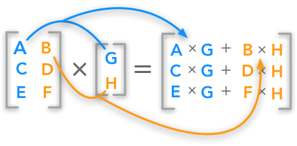
1.4.4. Matrix product

When both inputs are matrices, the operator @ performs a matrix multiplication. Specifically, given two matrices \(A\in\mathbb{R}^{M\times N}\) and \(B\in\mathbb{R}^{N\times K}\), their product is equal to the scalar product between the rows of \(A\) and the columns of \(B\):

\[\begin{split} AB = \begin{bmatrix} \_\!\_\; {\bf a}_1^\top \,\_\!\_ \\ \vdots\\ \_\!\_\; {\bf a}_M^\top \,\_\!\_ \\ \end{bmatrix} \begin{bmatrix} | & & |\\[-1em] {\bf b}_1 & \dots & {\bf b}_K\\ | & & |\\ \end{bmatrix} = \begin{bmatrix} {\bf a}_1^\top{\bf b}_1 & \dots & {\bf a}_1^\top{\bf b}_K\\ \vdots & & \vdots\\ {\bf a}_M^\top{\bf b}_1 & \dots & {\bf a}_M^\top{\bf b}_K \end{bmatrix}. \end{split}\]

X = np.array([[1,3,1],[2,5,1]])
Y = np.array([[5,1],[9,2],[14,1]])

Z = X @ Y

+-------+-----------+
|     X | [[1 3 1]  |
|       |  [2 5 1]] |
+-------+-----------+
|     Y | [[ 5  1]  |
|       |  [ 9  2]  |
|       |  [14  1]] |
+-------+-----------+
| X @ Y | [[46  8]  |
|       |  [69 13]] |
+-------+-----------+