4.6.5. Example 5

An optimization problem may sometimes require that the solution satisfies a specific condition. This scenario commonly known as constrained optimization is illustrated through the resolution of the following problem.

Problem

Find the dimensions of a closed cylinder with a volume of \(V=33\) cm3 and the minimum surface area.

4.6.5.1. Mathematical formulation

It is always recommended to begin the analysis of an optimization problem by sketching the situation. Since you are asked to build a closed cylinder, it is natural to draw each piece separately: the circular top, cylindrical side, and circular bottom. This is done in the picture below, where the height is denoted by the variable \(h\) and the radius by the variable \(r\). Excellent! You have identified the variables of the problem. Moving on.

4.6.5.1.1. Cost function

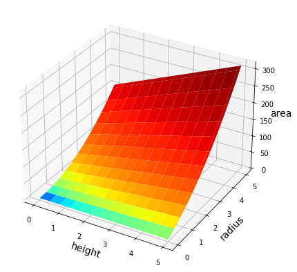
The next step is to write down a formula for the quantity you want to optimize. Most frequently you’ll use your everyday knowledge of geometry for this step. In the current example, you are looking for the values of \(h\) and \(r\) that will minimize the cylinder’s surface area. So, let’s write an equation for the total surface area as a function of the height and the radius:

\[\begin{split} \begin{aligned} J(h, r) &= A_{\rm top} + A_{\rm cylinder} + A_{\rm bottom} \\ &= \pi r^2 + 2\pi r h + \pi r^2 \\ &= 2\pi (r^2 + rh). \end{aligned} \end{split}\]

That’s it! You have written an equation for the quantity you want to minimize in terms of the relevant variables. Now, it is always useful to take a moment to analyze the function you just developed. Let’s plot the cost function to gain a better understanding of the problem. As you can see below, the surface area reduces more quickly by decreasing the radius rather than the height. That’s why the soda cans are shaped tall and narrow: it’s cheaper!

4.6.5.1.2. Constraint

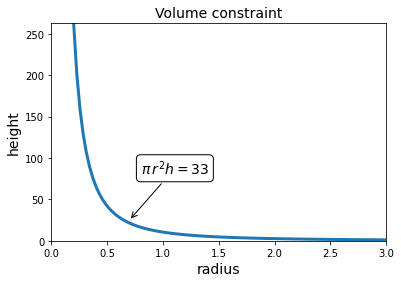
From the expression of the cost function, you clearly recognize that the minimum is attained at \(r=0\), which ironically implies that “the cheapest can is the one you never build”. To solve this paradox, you recall from the problem description that the can must hold exactly \(V=33\) cm3 of liquid. A cylinder of radius \(r\ge0\) and height \(h\ge0\) has a volume of

\[ V = \pi r^2 h. \]

This is the condition that the height and the radius must satisfy to be considered as possible solutions to the problem. Now, the solutions with \(r=0\) or \(h\le0\) are no longer acceptable, because they violate the volume constraint. Here is another reason why you often have constraints in optimization problems: to avoid trivial solutions! The figure below marks all the points \((h,r)\) satisfying the constraint for \(V=33\).

4.6.5.1.3. Optimization problem

Putting all together, the optimization problem can be written as

\[ \operatorname*{minimize}_{(h,r)\in\mathbb{R}_+^2}\quad 2\pi (r^2 + rh) \quad\textrm{subject to}\quad \pi r^2 h = V. \]

This formulation includes two terms.

• The function to be minimized. It is the term \(J(h,r) = 2\pi (r^2 + rh)\) expressing the total surface area of the cylinder as a function of its height \(h\) and its radius \(r\). It comes after the caption “minimize”.

• The constraint that the optimal solution must satisfy. It is the equation \(\pi r^2 h = V\) stating that the cylinder must have a volume of exactly \(V=33\) cm3. It comes after the caption “subject to”. The domain \(\mathbb{R}_+ = [0,+\infty[\) further indicates that the variables cannot take negative values.

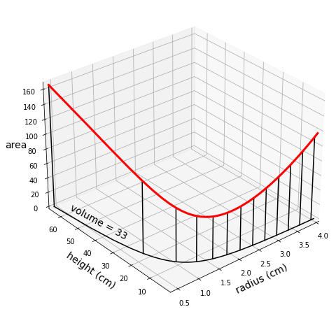
Although the cost function \(J(h,r)\) attains the lowest value at \((0,0)\), this is not the optimal solution because it does not satisfy the constraint. The optimal solution is the point attaining the smallest value of the function, among all the points satisfying the constraint. The figure below plots the function on the points respecting the constraint. You don’t care what happens elsewhere, because those other points should be never considered as possible candidates to solve the problem.

4.6.5.2. Problem solving

Once you defined the optimization problem, it is time to start thinking how to solve it. The major difficulty in your current formulation is given by the volume constraint. Nonconvex constraints are usually hard to deal with, but not this time luckily. There is a simple trick that you can use to reformulate your problem and get rid of this annoying constraint.

4.6.5.2.1. Remove the equality constraint

By looking at the points satisfying the volume constraint, you can notice they form a smooth curve where each radius \(r\) is mapped to a unique height \(h\). This happens because the constraint implictly defines the height as a function of the radius. There is a little trick to deal with such equality constraints. You can rewrite the equation so that one variable is expressed in terms of the others

\[ \pi r^2 h = V \qquad\implies\qquad h = \dfrac{V}{\pi r^2}. \]

This is a one-to-one mapping between the radius and the height, in the sense that every value \(h>0\) is associated to a unique value \(r>0\), and vice versa. Remember that the solutions to an optimization problem do not change if (some or all) the variables are transformed by a one-to-one mapping. More precisely, you can substitute the variable \(h\) in the cost function

\[ 2\pi (r^2 + rh) = 2\pi \left(r^2 + r \frac{V}{\pi r^2}\right) = 2\pi r^2 + \frac{2V}{r}. \]

This leads to an equivalent optimization problem that involves only the variable \(r\) over the open set of positive numbers

\[ \operatorname*{minimize}_{r>0}\quad 2\pi r^2 + \frac{2V}{r}. \]

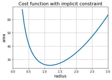
The substitution in the cost function ensures that the volume constraint is implicitly enforced, making it equivalent to the original problem. The reformulated cost function is shown in the figure below.

Note that the “substitution trick” cannot be always applied, because not every constraint defines an implicit function. For example, a common type of implicit function is the inverse function, but not all functions have a unique inverse function. The implicit function theorem provides conditions under which some kinds of relations define an implicit function. An implicit function can sometimes be successfully defined only after “zooming in” on some part of the constraint, and “cutting away” some unwanted branches. At other times, the implicit function cannot be written out explicitly as a closed-form expression, and a method called implicit differentation may be required to solve the optimization problem.

4.6.5.2.2. Analytical approach

Thanks to the substitution trick, you now have an “easy” optimization problem. What comes next is to find the minimum of the cost function

\[ A(r) = 2\pi r^2 + \frac{2V}{r}. \]

As the function \(A(r)\) is strongly convex, you can find the unique minimum by setting the derivative to zero, and solving the resulting equation

\[ A'(r) = 4\pi r - \frac{2V}{r^2} = 0. \]

By multiplying both sides of the equation by \(r^2\), you arrive at the cubic equation

\[ 4\pi r^3 - 2V = 0 \]

whose solution is the optimal radius

\[ r_* = \sqrt[3]{\frac{V}{2\pi}}. \]

Then, the optimal height can be deduced from the volume constraint, yielding

\[ h_* = \frac{V}{\pi r_*^2} = \frac{V}{\pi}\sqrt[3]{\frac{4\pi^2}{V^2}} = \sqrt[3]{\frac{4\pi^2 V^3}{\pi^3 V^2}} = \sqrt[3]{\frac{4 V}{\pi}} = 2 \sqrt[3]{\frac{V}{2\pi}} = 2 r_*. \]

Incidentally, you gained a nice insight by noticing that the optimal height is exactly twice the optimal radius!

4.6.5.2.3. Numerical approach

Alternatively, and even more so if the analytical approach is not practicable, you can approximate the solution to your problem with a numerical algorithm such as gradient descent. As in the previous exemple, you need to

• implement the cost function with NumPy operations supported by Autograd,

• select the initial point, the step-size, and the number of iterations.

You are then ready to run gradient descent.

volume = 33

def cost_fun(radius):
    return 2*np.pi * radius**2 + 2*volume / radius

init = [1.0]  # initialization
alpha = 0.01  # step-size
epochs = 100  # iterations

radius, history = gradient_descent(cost_fun, init, alpha, epochs)

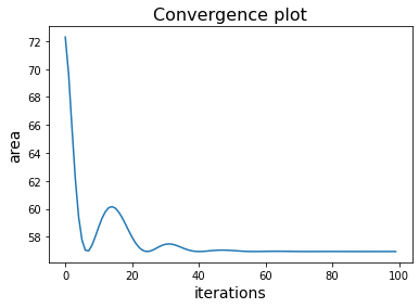
The figure below shows the convergence plot produced by gradient descent. Remark that the plot decreases and eventually flattens. This indicates that gradient descent successfully converged to the minimum.

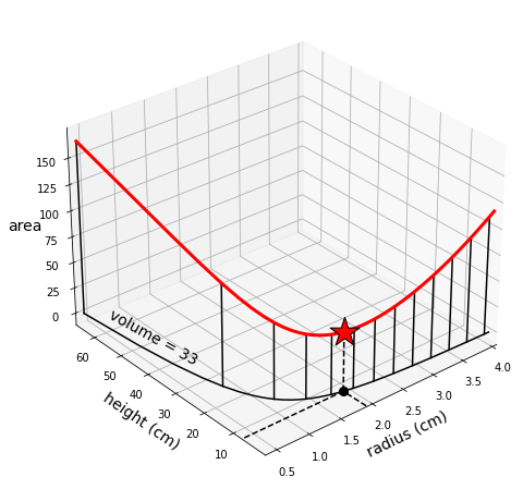
The following figure displays the optimal radius and height on the original cost function.