5.4.3. Simplex

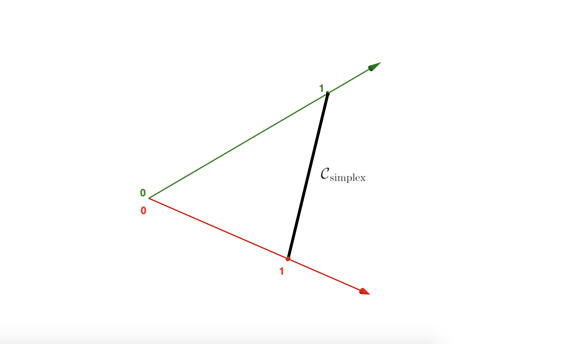
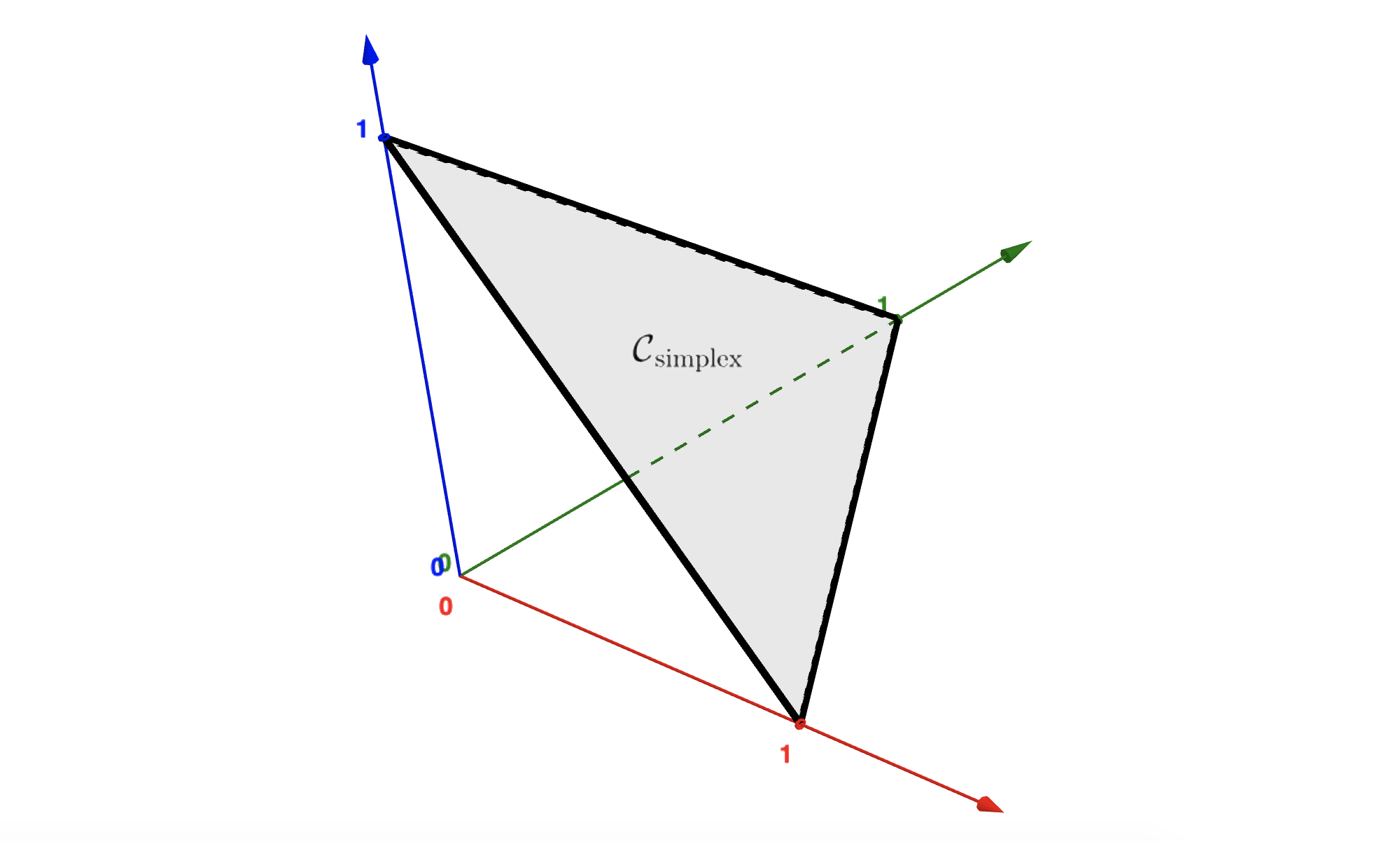
For a given scalar \(\xi\ge0\), the simplex is a linear constraint defined as

\[ \mathcal{C}_{\rm simplex} = \big\{ {\bf w} \in \mathbb{R}^{N} \;|\; {\bf w} \ge 0,\; {\bf 1}^\top {\bf w} = \xi \big\}, \]

where \({\bf 1}=[1\;\dots\;1]^\top \in \mathbb{R}^N\) is the vector with all elements to 1. The condition \(\xi \ge 0\) allows this subset to be nonempty. The figure below shows how this constraint looks like in \(\mathbb{R}^{2}\) or in \(\mathbb{R}^{3}\).

Simplex in 2D

Simplex in 3D

5.4.3.1. Constrained optimization

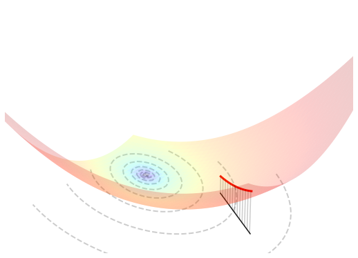
Optimizing a function \(J({\bf w})\) subject to the simplex can be expressed as

\[\begin{split} \operatorname*{minimize}_{\textbf{w}\in\mathbb{R}^N}\;\; J({\bf w}) \quad{\rm s.t.}\quad \begin{cases} {\bf w} \ge 0 \\ {\bf 1}^\top {\bf w} = \xi. \end{cases} \end{split}\]

The figure below visualizes such an optimization problem in \(\mathbb{R}^{2}\).

5.4.3.2. Orthogonal projection

The projection of a point \({\bf u}\in\mathbb{R}^{N}\) onto the simplex is the (unique) solution to the following problem

\[\begin{split} \operatorname*{minimize}_{{\bf w}\in\mathbb{R}^N}\;\; \|{\bf w}-{\bf u}\|^2 \quad{\rm s.t.}\quad \begin{cases} {\bf w} \ge 0 \\ {\bf 1}^\top {\bf w} = \xi. \end{cases} \end{split}\]

The solution can be computed as follows.

Projection onto the simplex

\[ \mathcal{P}_{\mathcal{C}_{\rm simplex}}({\bf u}) = \max\{{\bf 0},{\bf u} - \lambda{\bf 1}\} \]

The value \(\lambda \in \mathbb{R}\) is the unique solution of the equation

\[ \sum_{n=1}^N \max\{0,u_n-\lambda\} = \xi, \]

which can be easily determined in two steps:

• Sort \({\bf u}\) into \({\bf \tilde{u}}\) so that \(\tilde{u}_1 \ge \dots \ge \tilde{u}_N\),

• Set \(\lambda = \max_n\big\{(\tilde{u}_1+\dots+\tilde{u}_n - \xi) \,/\, n\big\}\).

Knapsack

A more general version of the simplex is called the knapsack:

\[ \mathcal{C}_{\rm knapsack} = \big\{ {\bf w} \in \mathbb{R}^{N} \;|\; {\bf a} \le {\bf w} \le {\bf b}\;{\rm and}\; {\bf c}^\top {\bf w} = d \big\}. \]

The projection onto this convex set is known as the continuous quadratic knapsack problem. If you ever need it, there exist numerical methods to efficiently compute this projection.

5.4.3.3. Implementation

The python implementation is given below.

def project_simplex(u, bound):
    
    assert bound >= 0, "The bound must be non-negative"
    
    s = np.sort(u.flat)[::-1]
    c = (np.cumsum(s) - bound) / np.arange(1, np.size(u)+1)
    # i = np.count_nonzero(c < s)
    # l = c[i-1]
    l = np.max(c)
    p = np.maximum(0, u - l)
    
    return p

Here is an example of use.

u = np.array([5, 4, 1, 3, 2, 6])

p = project_simplex(u, bound=8)

5.4.3.4. Proof

By using the Lagrange multipliers to remove the equality constraint, the projection onto the simplex is the (unique) solution to the following problem

\[ \operatorname*{minimize}_{{\bf w}\ge0}\;\sup_{\lambda\in\mathbb{R}}\; \frac{1}{2}\|{\bf w}-{\bf u}\|^2 + \lambda ({\bf 1}^\top {\bf w} - \xi). \]

Strong duality holds, because this is a convex problem with linear constraints. Hence, it can be equivalently rewritten as

\[ \operatorname*{maximize}_{\lambda\in\mathbb{R}}\;\inf_{{\bf w}\ge0}\; \frac{1}{2}\|{\bf w}-{\bf u}\|^2 + \lambda ({\bf 1}^\top {\bf w} - \xi). \]

Taking advantage of the element-wise separability, the inner minimization is solved by projecting \({\bf u} - \lambda {\bf 1}\) onto the non-negative orthant:

\[ {\bf w}^* = \max\{{\bf 0}, {\bf u} - \lambda {\bf 1}\}. \]

Setting to zero the gradient w.r.t. \(\lambda\), the outer maximization is attained by the scalar \(\lambda\) that solves the equation

\[ \begin{aligned} {\bf 1}^\top {\bf w}^* = \xi \quad\Leftrightarrow\quad {\bf 1}^\top \max\{{\bf 0}, {\bf u} - \lambda {\bf 1}\} = \xi \quad\Leftrightarrow\quad \sum_{n=1}^N \max\{0,u_n-\lambda\} = \xi. \end{aligned} \]

Without loss of generality, assume that \({\bf u}\) is sorted into \({\bf \tilde{u}}\) in descending order \(\tilde{u}_1 \ge \dots \ge \tilde{u}_N\), and define the solution \({\bf \tilde{w}}=\max\{{\bf 0}, {\bf \tilde{u}} - \lambda {\bf 1}\}\) using the same ordering as \({\bf \tilde{u}}\). Moreover, denote by \(\rho\in\{1,\dots,N\}\) the number of positive components in the solution, so that \(\tilde{w}_1 \ge \dots \ge \tilde{w}_\rho > 0\) and \(\tilde{w}_{\rho+i} = 0\) for every \(i\ge1\). The reordered solution is such that

\[ \begin{aligned} \sum_{n=1}^N \tilde{w}_n = \xi \quad\Leftrightarrow\quad \sum_{n=1}^N \max\{0, \tilde{u}_n -\lambda \} = \xi \quad\Leftrightarrow\quad \sum_{n=1}^\rho (\tilde{u}_n -\lambda) = \xi, \end{aligned} \]

from which we deduce

\[ \lambda = \frac{1}{\rho}\Big(\sum_{n=1}^\rho \tilde{u}_n - \xi\Big). \]

Hence, the index \(\rho\) is the key to the solution, and luckly there are only \(N\) possible candidates

\[ (\forall k\in\{1,\dots,N\})\quad \lambda_k = \frac{1}{k}\big(\sum_{i=1}^k \tilde{u}_i - \xi\big). \]

To evaluate such candidates, consider the function

\[ h(\gamma) = \sum_{n=1}^N \max\{0, \tilde{u}_n -\gamma\}, \]

which is equal to \(\xi\) at the optimal \(\lambda\). Evaluating this function on \(\lambda_k\) yields

\[ h(\lambda_k) = \sum_{n=1}^N \max\{0, \tilde{u}_n - \lambda_k\} = \sum_{n=1}^{\rho_k} (\tilde{u}_n - \lambda_k) = \sum_{n=1}^{\rho_k} \tilde{u}_n - \rho_k\lambda_k, \]

where \(\rho_k = \max\{n \,|\, \tilde{u}_n > \lambda_k\}\) is the number of times an element \(\tilde{u}_n\) is greater than \(\lambda_k\). A simple calculation shows that \(h(\lambda_k) = \xi\) if and only if \(\rho_k = k\), which is exactly how the optimal \(\lambda\) was defined. Hence, the sought index \(\rho\) can be determined as

\[ \rho = \max\{k \,|\, \tilde{u}_k > \lambda_k\}. \]

TODO: prove that \(\rho = \arg\max_k \lambda_k\).