Example 1

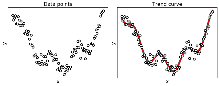
Let’s consider the problem of regression, that is the fitting of a representative curve to a given set of data points, as shown in the figure below. Regression in general may be performed for a variety of reasons: to produce a so-called trend curve that can be used to help visually summarize, drive home a particular point about the data under study, or to learn a model so that precise predictions can be made regarding output values in the future.

General approach

The data points for a regression problem come in the form of \(P\) input/output observation pairs

\[ \big({\bf x}^{(1)},y^{(1)}\big),\big({\bf x}^{(2)},y^{(2)}\big), \dots, \big({\bf x}^{(P)},y^{(P)}\big). \]

Note that the inputs \({\bf x}^{(p)}\) are vectors of length \(N\), whereas the outputs \(y^{(p)}\) are real numbers

\[\begin{split} {\bf x}^{(p)} = \begin{bmatrix} x_1^{(p)}\\ \vdots\\ x_N^{(p)} \end{bmatrix} \in \mathbb{R}^N \qquad\qquad y^{(p)}\in \mathbb{R}. \end{split}\]

The fundamental assumption is that the output \(y^{(p)}\) depends on the input \({\bf x}^{(p)}\) through an unknown relationship \(f\colon\mathbb{R}^N\to\mathbb{R}\) that is measurable in a noisy environment. Assuming the noise follows a normal distribution with zero mean and \(\sigma^2\) variance, this leads to the stochastic relationship

\[ y^{(p)} = f({\bf x}^{(p)}) + \varepsilon^{(p)} \qquad{\rm with}\qquad \varepsilon^{(p)}\sim \mathcal{N}(0,\sigma^2). \]

The idea is to approximate the unknown relationship with a parametric function that depends on some weights \({\bf w}\). Several models exist for this purpose, and they will be discussed in more detail later. Regardless of the chosen model, its parameters must be adjusted so that the following approximate equalities hold between the input/output data points

\[\begin{split} \begin{aligned} y^{(1)} &\approx \textsf{model}\left(\mathbf{x}^{(1)};\mathbf{w}\right)\\ y^{(2)} &\approx \textsf{model}\left({\bf x}^{(2)}; {\bf w}\right)\\ &\,\,\vdots\\ y^{(P)} &\approx \textsf{model}\left({\bf x}^{(P)}; {\bf w}\right). \end{aligned} \end{split}\]

Since the observed outputs are Gaussian distributed, it is statistically sound to minimize the mean square error between the observed outputs and model predictions at the given inputs, leading to the following optimization problem

\[ \operatorname*{minimize}_{{\bf w}}\quad \frac{1}{P}\sum_{p=1}^P \Big(\textsf{model}\left({\bf x}^{(p)}; {\bf w}\right) - y^{(p)}\Big)^2. \]

The cost function only depends on the parameters \({\bf w}\), because the data points are constant for a given regression task.

Linear model

To solve a regression problem, the parametric model must be precisely defined in mathematical terms. The simplest model imaginable is the hyperplane controlled by an intercept \(w_0\) and several slopes \(w_1,\dots,w_N\) (one for each input coordinate), yielding the linear relationship written as

\[ \textsf{linear-model}\left(\mathbf{x};\mathbf{w}\right) = w_{0} + w_1 x_1 + \dots + w_N x_N. \]

Solving a linear regression problem consists of finding the \(N+1\) weights \(\mathbf{w}=[w_0,w_1,\dots,w_N]^\top\) that minimize the mean square error between the observed outputs and the predictions of the linear model at the given inputs.

Example: one-dimensional linear model

In the running example, the inputs are scalar values (\(N=1\)), so the linear model boils down to

\[ \textsf{linear-model}(x;{\bf w}) = w_{0} + w_1 \, x .\]

Cost function

Note that the input vectors and the output scalars of a given dataset can be stacked into a matrix \({\bf X}\) and a vector \({\bf y}\) as follows

\[\begin{split} {\bf X} = \begin{bmatrix} 1 & x_1^{(1)} & \dots & x_N^{(1)}\\ 1 & x_1^{(2)} & \dots & x_N^{(2)}\\ \vdots & \vdots & \ddots & \vdots\\ 1 & x_1^{(P)} & \dots & x_N^{(P)}\\ \end{bmatrix} \in\mathbb{R}^{P\times(N+1)} \qquad\qquad {\bf y} = \begin{bmatrix} y^{(1)} \\ y^{(2)} \\ \vdots \\ y^{(P)}\\ \end{bmatrix} \in\mathbb{R}^{P}. \end{split}\]

The mean square error incurred by the linear moder over all the dataset can be written as

\[\begin{split} \begin{aligned} J({\bf w}) &= \frac{1}{P}\sum_{p=1}^P \Big(\textsf{linear-model}\left({\bf x}^{(p)}; {\bf w}\right) - y^{(p)}\Big)^2 \\[0.5em] &= \frac{1}{P} \left\|\begin{pmatrix} \textsf{linear-model}\left(\mathbf{x}^{(1)};\mathbf{w}\right) - y^{(1)}\\ \textsf{linear-model}\left(\mathbf{x}^{(2)};\mathbf{w}\right) - y^{(2)}\\ \vdots \\ \textsf{linear-model}\left(\mathbf{x}^{(P)};\mathbf{w}\right) - y^{(P)}\\ \end{pmatrix}\right\|^2 \\[0.5em] &= \frac{1}{P} \left\|\begin{pmatrix} w_{0} + w_1 x_1^{(1)} + \dots + w_N x_N^{(1)} - y^{(1)}\\ w_{0} + w_1 x_1^{(2)} + \dots + w_N x_N^{(2)} - y^{(2)}\\ \vdots \\ w_{0} + w_1 x_1^{(P)} + \dots + w_N x_N^{(P)} - y^{(P)}\\ \end{pmatrix}\right\|^2 \\[0.5em] &= \frac{1}{P} \|{\bf X} {\bf w} - {\bf y}\|^2. \end{aligned} \end{split}\]

This is a convex function with a unique minimum, provided that the matrix \({\bf X}\) is full column rank. It is also Lipschitz differentiable, because the Hessian matrix is constant, and thus the function curvature is upper bounded by the maximum eigenvalue

\[ L=\sup_{\bf w}\|\nabla^2 J({\bf w})\| = \frac{2}{P}\|{\bf X}^\top{\bf X}\|_2.\]

The choice of stepsize \(\alpha<2/L\) guarantees the convergence of gradient descent for solving this problem.

The figure below illustrates the process of solving the linear regression problem with gradient descent. The left panel shows how the linear model fits the data using the weights generated at the \(k\)-th iteration of gradient descent, whereas the right panel shows the convergence plot up to the \(k\)-th iteration. Pushing the slider to the right animates gradient descent from start to finish, with the best fit occurring at the end of the run, when the minimum of the cost function is being attained. Note that the linear model is a poor choice for this dataset, because the underlying relationship is clearly nonlinear.

Extended linear model

There is a simple trick to enhance the prediction capability of a linear model. It consists of taking a linear combination of simple nonlinear functions, whose number \(B\) is arbitrary fixed, yielding

\[ \textsf{extended-model}({\bf x},{\bf w}) = w_{0} + w_1 \, f_1({\bf x}) + \dots + w_B \, f_B({\bf x}). \]

When the functions \(f_b({\bf x})\) do not have internal parameters, this model remains linear with respect to the weights \(\mathbf{w}\). Nonetheless, the model can be made nonlinear with respect to \({\bf x}\) by appropriately choosing the functions \(f_b({\bf x})\). This kind of practice is referred to as feature engineering. An interesting choice is to use polynomial transformations, where each function \(f_b({\bf x})\) raises the input coordinates to the power of some values (possibly zero), such as

\[ f_b({\bf x}) = x_{1}^{d_{1,b}} \, x_{2}^{d_{2,b}} \,\dots\, x_{N}^{d_{N,b}}. \]

Just like before, the goal is to find the \(B+1\) weights \(\mathbf{w}=[w_0,w_1,\dots,w_B]^\top\) that minimize the mean square error between the observed outputs and the predictions of the extended model at the given inputs. Fortunately, this task is equivalent to solving a linear regression problem after a transformation of the input vectors.

Example: one-dimensional quadratic model

In the running example, it looks like the appropriate model is a quadratic polynomial, which can be obtained by setting \(B=2\), \(f_1(x)=x\), and \(f_2(x)=x^2\). This yields

\[ \textsf{quadratic-model}(x,{\bf w}) = w_{0} + w_1 \, x + w_2 \, x^2. \]

Cost function

Note that the transformed input vectors can be stacked into the matrix

\[\begin{split} {\bf X}_{\bf f} = \begin{bmatrix} 1 & f_1({\bf x}^{(1)}) & \dots & f_B({\bf x}^{(1)})\\ 1 & f_1({\bf x}^{(2)}) & \dots & f_B({\bf x}^{(2)})\\ \vdots & \vdots & \ddots & \vdots\\ 1 & f_1({\bf x}^{(P)}) & \dots & f_B({\bf x}^{(P)})\\ \end{bmatrix} \in\mathbb{R}^{P\times(B+1)}. \end{split}\]

The mean square error incurred by the extended linear moder over all the dataset can be written as

\[ J({\bf w})=\frac{1}{P}\|{\bf X}_{\bf f} {\bf w} - {\bf y}\|^2. \]

This is a convex function with a unique minimum, provided that the matrix \({\bf X}_{\bf f}\) is full column rank. It is also Lipschitz differentiable with constant

\[ L= \frac{2}{P}\|{\bf X}_{\bf f}^\top{\bf X}_{\bf f}\|_2. \]

The choice of stepsize \(\alpha<2/L\) guarantees the convergence of gradient descent for solving this problem.

The figure below illustrates the process of solving the polynomial regression problem with gradient descent. The left panel shows how the quadratic model fits the data using the weights generated at the \(k\)-th iteration of gradient descent, whereas the right panel shows the convergence plot up to the \(k\)-th iteration. Pushing the slider to the right animates gradient descent from start to finish, with the best fit occurring at the end of the run, when the minimum of the cost function is being attained. Note that the quadratic model does a good job at capturing the general trend of the data points.

Universal nonlinear model

The fundamental issue with the extended linear model is the difficulty of feature engineering, because it strongly depends on the level of knowledge regarding the problem under study. This motivates an alternative approach known as feature learning, whose goal is to automate the process of identifying appropriate nonlinear features for arbitrary datasets. Doing so requires a manageable collection of universal approximators, of which three strains are popularly used: fixed-shape approximators, neural networks, or decision trees. As for the neural networks, the universal nonlinear model is defined as a linear combination of nonlinear functions, whose number \(B\) is arbitrary fixed, yielding

\[ \textsf{nonlinear-model}({\bf x},\,{\bf w}_0, {\bf w}_1, \dots, {\bf w}_B) = w_{00} + w_{01} \, g({\bf x}, \mathbf{w}_1) + \dots + w_{0B} \, g({\bf x}, \mathbf{w}_B). \]

The peculiarity of such model is that each term \(g({\bf x}, \mathbf{w}_b)\) depends on its own set of parameters \(\mathbf{w}_b\). In the context of neural networks, a popular nonlinear term is the rectified linear function (relu) defined as

\[\begin{split} \begin{aligned} g({\bf x}, \mathbf{w}_b) &= \max\big\{0,w_{b0} + w_{b1} x_1 + \dots + w_{bN} x_N\big\}. \\ %&\;{\rm or}\\ %g({\bf x}, \mathbf{w}_b) &= \tanh\big(w_{b0} + w_{b1} x_1 + \dots + w_{bN} x_N\big). \end{aligned} \end{split}\]

Solving a nonlinear regression problem consists of finding the \((N+2)B+1\) weights \(\mathbf{w}=({\bf w}_0, {\bf w}_1, \dots, {\bf w}_B)\) that minimize the mean square error between the observed outputs and the predictions of the nonlinear model at the given inputs.

Example: one-dimensional nonlinear model

In the running example, the inputs are scalar values (\(N=1\)), so the universal nonlinear model boils down to

\[ \textsf{nonlinear-model}({\bf x},{\bf w}) = w_{00} + w_{01} \, \max\{0,w_{10} + w_{11} \, x\} + \dots + w_{0B} \, \max\{0,w_{B0} + w_{B1} \, x\}. \]

Cost function

Note that the internal parameters can be stacked into the matrix

\[ {\bf W} = \begin{bmatrix} {\bf w}_1 & {\bf w}_2 & \dots & {\bf w}_B \end{bmatrix} \in\mathbb{R}^{(N+1)\times B} \]

and the intermediate features can be stacked into the matrix

\[\begin{split} {\rm relu}({\bf X}{\bf W}) = \begin{bmatrix} 1 & \max\big\{0,{{\bf x}^{(1)}}^\top {\bf w}_1\big\} & \dots & \max\big\{0,{{\bf x}^{(1)}}^\top {\bf w}_B\big\} \\ 1 & \max\big\{0,{{\bf x}^{(2)}}^\top {\bf w}_1\big\} & \dots & \max\big\{0,{{\bf x}^{(2)}}^\top {\bf w}_B\big\} \\ \vdots & \vdots & \ddots & \vdots\\ 1 & \max\big\{0,{{\bf x}^{(P)}}^\top {\bf w}_1\big\} & \dots & \max\big\{0,{{\bf x}^{(P)}}^\top {\bf w}_B\big\} \\ \end{bmatrix} \in\mathbb{R}^{P\times(B+1)}. \end{split}\]

The mean square error incurred by the nonlinear moder over all the dataset can be written as

\[ J({\bf w}) = \frac{1}{P}\sum_{p=1}^P \Big(\textsf{nonlinear-model}\left({\bf x}^{(p)},{\bf w}\right) - y^{(p)}\Big)^2 = \frac{1}{P}\big\|{\rm relu}({\bf X}{\bf W}){\bf w}_0 - {\bf y}\big\|^2. \]

This is a nonconvex function with multiple local minima, which can be optimized by gradient descent.

The figure below illustrates the process of solving the nonlinear regression problem with gradient descent. The left panel shows how the nonlinear model fits the data using the weights generated at the \(k\)-th iteration of gradient descent, whereas the right panel shows the convergence plot up to the \(k\)-th iteration. Pushing the slider to the right animates gradient descent from start to finish, with the best fit occurring at the end of the run, when the minimum of the cost function is being attained. Note that the nonlinear model does a great job at capturing the relationship underlying the data points.