4.6.1. Example 1

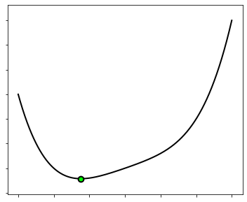
Consider this optimization problem involving a convex function of one variable

\[ \operatorname*{minimize}_{w\in\mathbb{R}}\quad \frac{1}{10}\big( w^4 + w^2 + 10w\big). \]

The cost function is shown below, where its minimum is marked with a green dot.

4.6.1.1. Analytical approach

When facing an optimization problem, the first question to ask is whether the minimum can be expressed in closed-form. To do this, you should recall the first-order optimality condition introduced at the beginning of this chapter, which characterizes the stationary points of a function as the solution(s) to a nonlinear system of equations. In this specific case, the cost function is convex, so the first-order optimality condition becomes a logical equivalence:

\[ \bar{w} = \operatorname*{argmin}_{w\in\mathbb{R}}\; \frac{1}{10}\big(\underbrace{w^4 + w^2 + 10w}_{J(w)} \big)\qquad\Leftrightarrow\qquad \underbrace{4 \bar{w}^3 + 2 \bar{w} + 10}_{J'(\bar{w})} = 0.\]

It is well known that a cubic equation has three possible roots, one of which is the sought minimum

\[ \bar{w} = \sqrt[3]{\frac{\sqrt{2031}-45}{36}} - \sqrt[3]{\frac{1}{6\left(\sqrt{2031}-45\right)}}. \]

A quick way to check this result is through the web site wolfram alpha.

4.6.1.2. Numerical approach

Gradient descent can be regarded as a numerical method for computing a close approximation of the exact solution \(\bar{w}\). This illustrates the general principle that optimization problems can be solved without going through the analytical approach, which is however impossible to enact in many circumstances.

To run gradient descent, you first implement the cost function with NumPy operations supported by Autograd. You may indifferently use the lambda keyword or the standard def declaration.

cost_fun = lambda w: (w**4 + w**2 + 10*w) / 10

Then, you select an initial point, the step-size, and the number of iterations. There is no specific policy that guides the choice of these parameters. But do not worry about it right now: you will learn the best practices in the next chapter!

init = [2.5]  # initial point
alpha = 0.1   # step-size
epochs = 50   # number of iterations

You are now ready to run gradient descent.

w, history = gradient_descent(cost_fun, init, alpha, epochs)

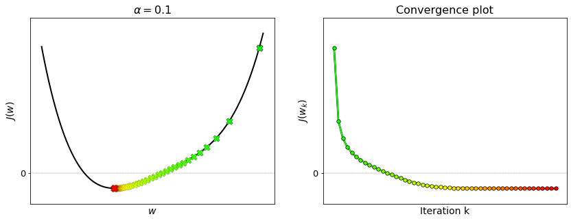
The figure below shows the sequence of points generated by gradient descent to minimize the cost function. At each iteration, the current point is marked on the function with a green cross at the initial point, a yellow cross as the algorithm converges, and a red cross at the final point. The same color scheme is used in the convergence plot. Remark that the convergence plot decreases and eventually flattens. This indicates that gradient descent has converged to the minimum.

4.6.1.3. Vanishing derivatives

Remark that the algorithm slows down considerably as it approaches the minimum of the function. This is due to the fact that the first derivative shrinks to zero near the solution, namely \(J'(w) \to 0\) as \(w\to\bar{w}\). Such feature is essential to guarantee the convergence. Thanks to it, gradient descent acquires the ability to stop exactly at the solution.

The widget below animates the process of gradient descent applied to minimize this function. Moving the slider visualizes the sequence of points generated by the algorithm, along with the tengent line at each point. By pushing the slider all the way to the right, you can remark that the tangent gradually reduces its slope, until it gets completely flat at the minimum.