2.6. Stochastic optimization

Grid search and random search incarnate two opposite philosophies: the former performs global optimization, whereas the latter performs local optimization. Both approaches have their unique advantages and weaknesses. Grid search is capable of finding the global minimum of a function even if the latter presents many local minima, but the result can be extremely inaccurate when the sampling is done wrong. On the other side, random search is efficient and accurate, but it may converge to a local minimum depending on the initialization. To combine the strengths of both approaches, there exist several hybrid approaches that sit in between global and local optimization. In this section, we will focus on stochastic optimization and we will discuss one specific strategy in more detail, which is called the cross-entropy method.

2.6.1. General approach

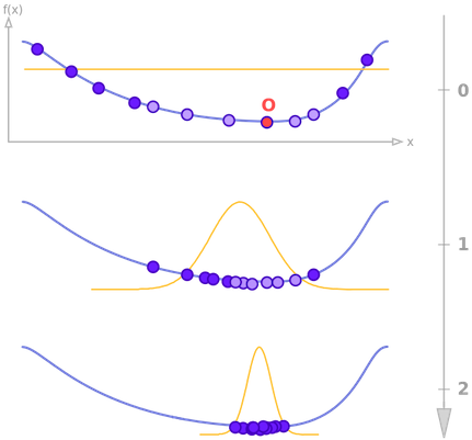
Stochastic optimization guides the search for the optimum by building and sampling explicit probabilistic models of promising candidate solutions. Optimization is viewed as a series of incremental updates of a probabilistic model, starting with the model encoding an uninformative prior, and ending with the model that generates only the global optima. The process is illustrated in the figure below. At each iteration, a random selection (blue points) is performed in accordance to a probability distribution (orange line), which is then updated using a subset of sampled points (light blue points). This is repeated several times, producing a sequence of distributions that gradually puts all its mass on a minimum of the function.

Stochastic optimization belongs to the class of evolutionary algorithms, which also include genetic algorithms, evolution strategies, swarm intelligence, and Monte Carlo methods such as simulated annealing. The main difference with classic evolutionary algorithms is that the latter generate new candidate solutions using an implicit distribution defined by one or more variation operators. On the contrary, stochastic optimization uses an explicit probability distribution encoded by a multivariate probability distribution (or a Bayesian network).

2.6.2. Cross-entropy method

The cross-entropy method is a Monte Carlo technique for importance sampling and optimization, applicable to both combinatorial and continuous problems. It works by repeating the three following steps.

• Draw samples from a normal distribution.

• Compute the mean and variance of those samples attaining the lowest values on the fuction.

• Update the distribution parameters to produce a better sampling in the next iteration.

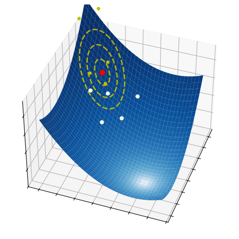
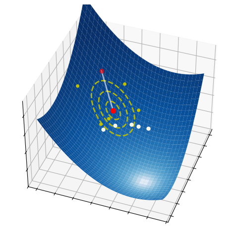
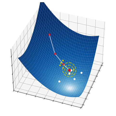
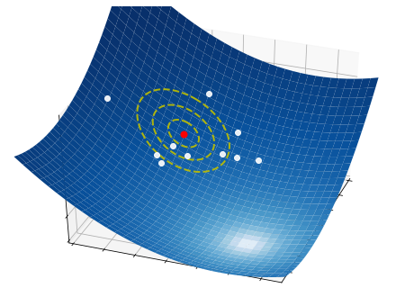
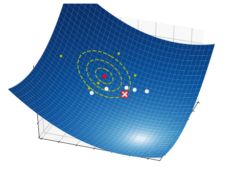
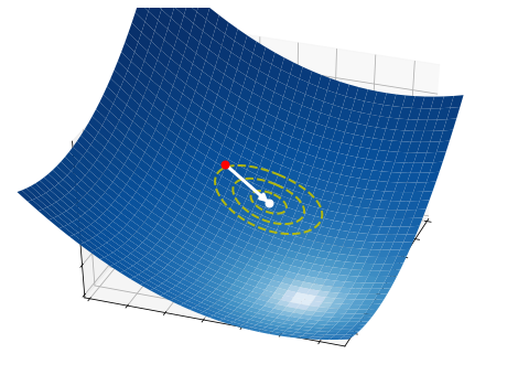
These three simple steps lead to a surprisingly effective optimization method. They are illustrated in the pictures below on a two-dimensional function. At each iteration, a number of samples are drawn from a normal distribution (red circle and dashed yellow lines). A small subset of these points is selected, precisely those attaining the smallest values of the fuction (white dots). The mean and the variance of such a subset are then used to update the current distribution (white arrow).

Iteration 1

Iteration 2

Iteration 3

Iteration 4

2.6.2.1. Step 1 - Sampling

How do we represent a probability distribution? The idea is to mantain two vectors \({\bf \mu}_k\) and \({\bf \sigma}_k\) representing the means and variances of a multivariate normal distribution, which is used to draw the samples at each iteration \(k\):

\[ \widehat{ {\bf w} }_k^{(1)}, \dots, \widehat{ {\bf w} }_k^{(S)} \sim \mathcal{N}\big({\bf \mu}_k, {\rm diag}({\bf \sigma}_k^2 + \epsilon)\big). \]

Note that a small extra variance \(\epsilon\ge0\) may be added to ensure continual exploration.

2.6.2.2. Step 2 - Estimation

Once the candidate points are sampled, we sort them according to the respective function values:

\[ J\big(\widehat{ {\bf w} }_k^{(i_1)}\big) \le \dots \le J\big(\widehat{ {\bf w} }_k^{(i_B)}\big) \le \dots \le J\big(\widehat{ {\bf w} }_k^{(i_S)}\big). \]

Then, we compute the mean and standard deviation of the first \(B\) samples:

\[ \overline{ {\bf \mu} }_k = \frac{1}{B} \sum_{b=1}^B \widehat{ {\bf w} }_k^{(i_b)} \qquad \qquad \overline{ {\bf \sigma} }_k = \sqrt{\frac{1}{B-1}\sum_{b=1}^B \big(\widehat{ {\bf w} }_k^{(i_b)} - \overline{ {\bf \mu} }_k \big)^2}. \]

2.6.2.3. Step 3 - Update

Finally, we update the parameters of the normal distribution with an exponential moving average:

\[\begin{split}\begin{cases} {\bf \mu}_{k+1} = \alpha \, \overline{\bf \mu}_k + (1-\alpha) \, {\bf \mu}_{k} \\ {\bf \sigma}_{k+1} = \alpha \, \overline{\bf \sigma}_k + (1-\alpha) \, {\bf \sigma}_{k} \end{cases}\end{split}\]

where \(\alpha\in(0,1]\) is a small constant. Then, the process starts over from the first step, using the new set of parameters \({\bf \mu}_{k+1}\) and \({\bf \sigma}_{k+1}\).

2.6.3. Numerical implementation

The following is a Python implementation of the cross-entropy method. Notice that each step of the algorithm is translated into one or several lines of code. Numpy library is used to vectorize operations whenever possible.

def cross_entropy_method(cost_fun, w_init, alpha, epochs, n_points):
    """
    Finds the minimum of a function.
    
    Arguments:
    cost_fun -- cost function | callable that takes 'w' and returns 'J(w)'
    w_init   -- initial point | vector of shape (N,)
    alpha    -- step-size     | scalar between 0 and 1
    epochs   -- n. iterations | integer
    n_points -- n. directions | integer
    
    Returns:
    w -- minimum point | vector of shape (N,)
    """
    
    # Internal settings
    n_elites = int(n_points * 0.2)
    init_std = 5.0
    
    # Probability distribution
    mean = np.array(w_init, dtype=float).ravel()  # vector (1d array)
    std  = np.ones_like(mean) * init_std

    # Iterative refinement
    for k in range(epochs):

        # Step 1. Draw random points
        points = mean + std * np.random.randn(n_points, std.size)

        # Step 2. Select the elites
        idx = np.argsort([cost_fun(w) for w in points], axis=None)
        idx = idx[:n_elites]
        elites = points[idx]

        # Step 3. Update the distribution
        mean = (1-alpha) * mean + alpha * elites.mean(axis=0)
        std  = (1-alpha) * std  + alpha * elites.std(axis=0)

    return mean

The python implementation requires five arguments:

• the function to optimize,

• a starting point,

• a step-size that controls the update of parameters,

• the number of iterations to be performed,

• the number of samples per iteration.

An usage example is presented next.

# cost function of two variables
cost_fun = lambda w: (2*w[0]+1)**2 + (w[1]+2)**2

w_init = [1, 3]  # initialization
alpha  = 0.2     # step-size
epochs = 20      # number of iterations
n_points = 50    # number of samples per iteration

w = cross_entropy_method(cost_fun, w_init, alpha, epochs, n_points)

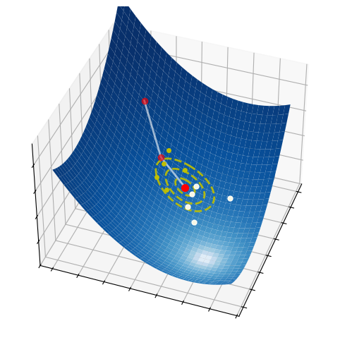
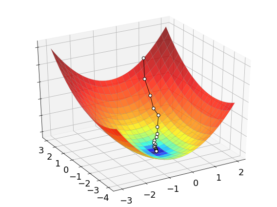
The process of optimizing a function with the cross-entropy method is illustrated below. The white dots mark the sequence of points generated by the algorithm to find its final approximation of the minimum. While these points may seem to be much less than grid search, keep in mind that the cross-entropy method tests a bunch of points at each iteration. These points are not shown in the picture, but they definitely contribute to the overall complexity of the method.

2.6.4. Discussion

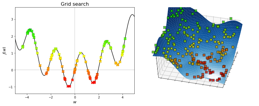
Let us compare grid search, random search, and the cross-entropy method on the following functions.

\[\begin{split} \begin{aligned} (\forall w\in\mathbb{R})\qquad J(w) &= \sin(3w) + 0.1 w^2 \\ (\forall {\bf w}\in\mathbb{R}^2)\qquad J({\bf w}) &= \|A{\bf w}\|^2 - \frac{1}{2} \big(\cos(2\pi \, {\bf a}_1^\top {\bf w}) + \cos(2\pi \, {\bf a}_2^\top {\bf w})\big) \end{aligned} \end{split}\]

The figures below display the points generated by grid search. The algorithm is theoretically able to find the global minimum, provided that enough points are being searched. Therefore, sampling is important to grid search.

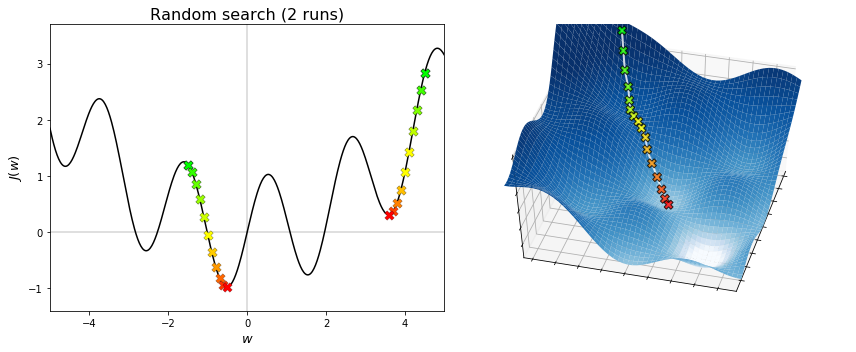
The figures below display the sequences generated by random search. The algorithm converges to the minimum that is nearest to the initial point, regardless of whether it is global or local. Therefore, initialization is important to local search.

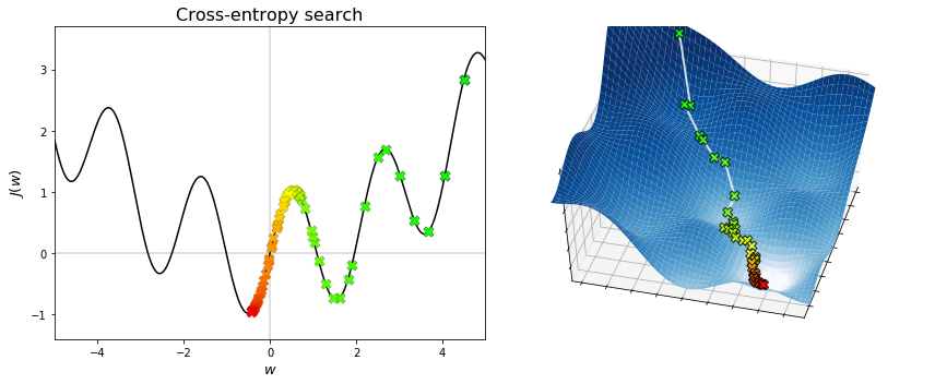
The figures below display the sequences generated by the cross-entropy method. The algorithm is capable of converging to the global minimum, without getting stuck into any local minima. To do this, a fairly amount of points needs to be searched at each iteration. Hence, the cross-entropy method overcomes the limitations of grid search and random search, but at the expense of increasing the amount of sampling. Note also that the convergence to a global minimum is still not guaranted. Indeed, when the algorithmic parameters are poorly chosen, the probability distribution may shrink too early and put all its mass on a point that is not optimal (neither globally nor locally). This undesired behaviour may be fought by adding a small extra variance in the sampling step, which however reduces the accuracy of the solution if chosen too large.

Beside the cross-entropy method, there exist many other stochastic optimization algorithms. One such example is the covariance matrix adaptation evolution strategy (CMA-ES), which has been designed to deal with difficult (non-convex, ill-conditioned, multi-modal, noisy) black-box optimization problems in continuous domain. It is considered the state-of-the-art in evolutionary computation, and one of the standard tools for continuous optimization. Several python implementations of this algorithm are available (CMA-ES/pycma). When you need to solve a black-box continuous optimization problem, CMA-ES should be your first choice!