5.2. Normal cone

The normal cone is a powerful concept that formally describes the geometrical situation where “a vector is orthogonal to a set”. As shown later in this chapter, combining the normal cone with the gradient of a function allows to characterize optimality in constrained optimization. But this section deals with defining the normal cone independently of optimization.

5.2.1. Informal definition

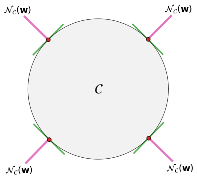
The normal cone of a subset \(\mathcal{C}\subset\mathbb{R}^N\) at a point \({\bf w}\in\mathbb{R}^N\) is the set of vectors orthogonal to \(\mathcal{C}\) around \({\bf w}\). The orthogonality is intended in a broad sense: a normal vector forms an angle of at least \(90°\) with all the directions [1] originating at \({\bf w}\), and oriented either to the interior of \(\mathcal{C}\) or tangentially with respect to \(\mathcal{C}\). The normal cone thereby depends on both the topology of \(\mathcal{C}\) and the point \({\bf w}\). Since the notions of orthogonality and tangency make only sense at the boundary of \(\mathcal{C}\), the normal cone is empty at the exterior of \(\mathcal{C}\), and it just contains the zero vector at the interior of \(\mathcal{C}\). This yields the following informal definition.

Normal cone

\[\begin{split} \mathcal{N}_{\mathcal{C}}({\bf w}) = \begin{cases} \emptyset & \textrm{if ${\bf w} \notin \mathcal{C}$}\\ \{{\bf 0}\} & \textrm{if ${\bf w} \in {\rm int}(\mathcal{C})$}\\ \{{\bf 0}\}\cup\{{\bf d}\in\mathbb{R}^N \,|\, \textrm{${\bf d}$ is orthogonal to $\mathcal{C}$ at ${\bf w}$} \} & \textrm{otherwise} \end{cases} \end{split}\]

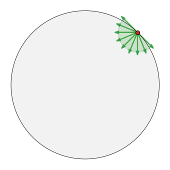
The figure below shows the normal cone at variour points of a set with a smooth boundary. For a given point marked in red, the pink area denotes all the directions orthogonal to the set, where the orthogonality is intended with respect to the tangent line marked in green. The pink area is the normal cone! For any point in the interior of the set, the normal cone only contains the vector \({\bf 0}\), because there is no orthogonal direction there.

5.2.2. Geometrical construction

There is a simple procedure for drawing the normal cone of a subset of \(\mathbb{R}^2\).

• Suppose you are given a set \(\mathcal{C}\subset \mathbb{R}^2\) and a point \({\bf w}\in\mathbb{R}^2\) at the boundary of \(\mathcal{C}\).

  • If \({\bf w}\) is at the interior or the exterior of \(\mathcal{C}\), the answer is trivial.

• Draw two vectors originating at \({\bf w}\) and oriented tangentially with respect to the boundary of \(\mathcal{C}\).

  • How to draw a tangent direction? Imagine a unit vector oriented from \({\bf w}\) to a point on the boundary of \(\mathcal{C}\). Move this point along the boundary by bringing it closer and closer to \({\bf w}\). When these two points coincide, the unit vector that you got is a tangent direction.

• Draw a half-line from \({\bf w}\) to the outside of \(\mathcal{C}\) and oriented at 90° to a tangent direction. Draw another half-line using the other tangent direction as a reference. The space between the half-lines is the normal cone at \({\bf w}\).

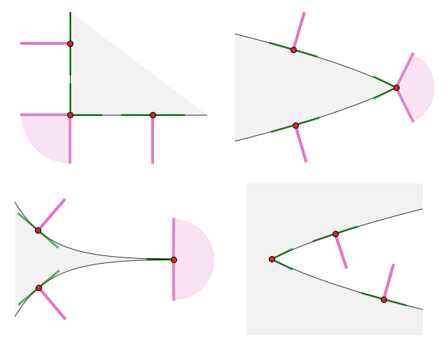
The figures below illustrate several examples of normal cone. [2]

5.2.3. Appendix: Rigorous definitions

The informal definition of normal cone is useful to grasp the basic idea. But it is rather vague, especially at the points where the boundary of \(\mathcal{C}\) is nonsmooth. A more general treatement relies on the notion of tangent cone. Loosely speaking, the tangent cone of \(\mathcal{C}\) at a point \({\bf w}\in\mathcal{C}\) is the set of all directions originating at \({\bf w}\), and oriented either to the interior of \(\mathcal{C}\), or tangentially with respect to \(\mathcal{C}\). It can thus be regarded as the union of feasible directions and tangent directions. Depending on the chosen point \({\bf w}\in\mathcal{C}\), there may exist either no feasible direction or no tangent direction, and there is neither one at exterior points of \(\mathcal{C}\). This yields the following informal definition. [1]

Tangent cone

\[\begin{split} \mathcal{T}_{\mathcal{C}}({\bf w}) = \begin{cases} \emptyset & \textrm{if ${\bf w} \notin \mathcal{C}$}\\[0.5em] \big\{\textrm{feasible directions of $\mathcal{C}$ at ${\bf w}$}\big\} \cup \big\{\textrm{tangent directions of $\mathcal{C}$ at ${\bf w}$}\big\} & \textrm{if ${\bf w} \in \mathcal{C}$} \end{cases} \end{split}\]

This appendix will formally define the feasible and the tangent directions, as well as the tangent and the normal cones.

5.2.3.1. Feasible direction

A feasible direction is a vector \({\bf d}\in \mathbb{R}^N\) such that the shifted point \({\bf w} + \alpha \, {\bf d}\) belongs to \(\mathcal{C}\) for all sufficiently small \(\alpha\ge0\):

\[ \textrm{${\bf d}$ is a feasible direction of $\mathcal{C}$ at ${\bf w}$}\quad\Leftrightarrow\quad (\exists \delta>0:\forall \alpha\in[0,\delta])\quad {\bf w} + \alpha \, {\bf d}\in \mathcal{C}. \]

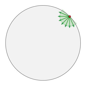
The figure below shows the feasible directions (green wedge/arrows) at a point on the boundary of a set \(\mathcal{C}\). Note that they are always oriented toward the interior of \(\mathcal{C}\). This is why no feasible direction exists when the interior of \(\mathcal{C}\) is empty, or when a point is located at the exterior of \(\mathcal{C}\). Conversely, all directions are feasible at a point located in the interior of \(\mathcal{C}\).

5.2.3.2. Tangent direction

A tangent direction is a vector \({\bf d}\in \mathbb{R}^N\) directly proportional to a unit vector oriented from \({\bf w}\) to a point \({\bf w}_k\) on the boundary of \(\mathcal{C}\) under the limit \({\bf w}_k \to {\bf w}\):

\[ \textrm{${\bf d}$ is a tangent direction of $\mathcal{C}$ at ${\bf w}$}\quad\Leftrightarrow\quad (\exists \{{\bf w}_k\} \subset \partial\mathcal{C} : {\bf w}_k\to{\bf w})\quad {\bf d} \propto \lim_{{\bf w}_k\to{\bf w}} \frac{{\bf w}_k-{\bf w}}{\|{\bf w}_k-{\bf w}\|}. \]

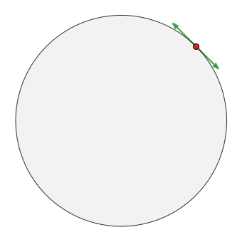
The figure below shows the tangent directions (green arrows) at a point on the boundary of a given set \(\mathcal{C}\). Note that they are always oriented tangentially to \(\mathcal{C}\). For this reason, no tangent direction exists at the exterior or at the interior of \(\mathcal{C}\). They only occur at the boundary of \(\mathcal{C}\), here denonted by \(\partial\mathcal{C}\).

5.2.3.3. Tangent cone

In the definition of tangent directions, it is possible to incorporate the feasible directions by replacing the boundary \(\partial\mathcal{C}\) with the whole \(\mathcal{C}\) itself. This yields the formal definition of tangent cone, which includes all the directions \({\bf d}\in \mathbb{R}^N\) directly proportional to a unit vector oriented from \({\bf w}\) to a point \({\bf w}_k\in\mathcal{C}\) under the limit \({\bf w}_k \to {\bf w}\):

\[ \mathcal{T}_{\mathcal{C}}({\bf w}) = \Big\{\alpha{\bf d}\in \mathbb{R}^N \;|\; \alpha\ge0,\; (\exists \{{\bf w}_k\} \subset \mathcal{C} : {\bf w}_k\to{\bf w})\quad {\bf d} = \lim_{{\bf w}_k\to{\bf w}} \frac{{\bf w}_k-{\bf w}}{\|{\bf w}_k-{\bf w}\|}\Big\}. \]

By definition, the tangent cone is closed. Note also that if a vector belongs to the tangent cone, then so is the vector scaled by any non-negative factor. This explains why \(\mathcal{T}_{\mathcal{C}}({\bf w})\) is a cone. Moreover, the tangent cone is empty at the exterior of \(\mathcal{C}\), whereas it reverts to \(\mathbb{R}^N\) at the interior of \(\mathcal{C}\). Hence it is only of interest at the boundary of \(\mathcal{C}\), as summarized below.

\[\begin{split} \begin{aligned} {\bf w} \notin \mathcal{C} \quad&\Rightarrow\quad \mathcal{T}_{\mathcal{C}}({\bf w}) = \emptyset\\[0.5em] {\bf w} \in {\rm int}(\mathcal{C}) \quad&\Rightarrow\quad \mathcal{T}_{\mathcal{C}}({\bf w}) = \mathbb{R}^N\\[0.5em] {\bf w} \in \partial\mathcal{C} \quad&\Rightarrow\quad \mathcal{T}_{\mathcal{C}}({\bf w}) \subset \mathbb{R}^N \end{aligned} \end{split}\]

Note

• No tangent direction exists at the exterior or at the interior of \(\mathcal{C}\).

• No feasible direction exists at the exterior of \(\mathcal{C}\) or when the interior of \(\mathcal{C}\) is empty.

• All directions are feasible at the interior of \(\mathcal{C}\).

The figure below shows an example of tangent cone. The feasible directions and the tangent directions are explicitly represented by the green wedge and the green arrows. Note in particular that the feasible directions are important to clarify the “correct side” of the tangent cone, which is never oriented outward the set \(\mathcal{C}\).

Convexity of the tangent cone

The tangent cone \(\mathcal{T}_{\mathcal{C}}({\bf w})\) is included in the closure of directions \(\alpha({\bf w} - {\bf u})\) such that \({\bf u}\in\mathcal{C}\) and \(\alpha\ge0\), yielding

\[ \mathcal{T}_{\mathcal{C}}({\bf w}) \subseteq {\rm closure}\big(\big\{{\bf d}\in \mathbb{R}^N \;|\; {\bf w} + \alpha{\bf d} \in \mathcal{C},\; \alpha\ge0\big\}\big). \]

Interestingly, the identity holds when \(\mathcal{C}\) is convex, and the tangent cone is itself convex

\[ \textrm{$\mathcal{C}\,$ is convex} \quad\Rightarrow\quad \textrm{$\mathcal{T}_{\mathcal{C}}({\bf w})$ is convex}. \]

When \(\mathcal{C}\) is nonconvex, hovewer, the tangent cone \(\mathcal{T}_{\mathcal{C}}({\bf w})\) may be nonconvex. For example, the nonconvex set \(\mathcal{C}=\{(x,y)\in\mathbb{R}^2\,|\, x^2 \le y^2\}\) has a nonconvex tangent cone in \((0,0)\).

5.2.3.4. Normal cone

The normal cone of \(\mathcal{C}\) at \({\bf w}\) is the set containing both the vector \({\bf 0}\) and all the vectors whose angle is at least \(90°\) with respect to any direction in the tangent cone of \(\mathcal{C}\) at \({\bf w}\):

\[\begin{split} \mathcal{N}_{\mathcal{C}}({\bf w}) = \begin{cases} \emptyset & \textrm{if ${\bf w} \notin \mathcal{C}$}\\[0.5em] \Big\{{\bf d}\in\mathbb{R}^N \;\big|\;\big(\forall {\bf t}\in\mathcal{T}_{\mathcal{C}}({\bf w})\big)\quad \underbrace{{\bf d}^\top {\bf t}\le 0}_{\scriptsize\begin{smallmatrix}{\rm angle}({\bf d},\,{\bf t})\,\ge\,90°\\{\rm or}\\{\bf d}=0\end{smallmatrix}}\Big\} & \textrm{if ${\bf w} \in \mathcal{C}$}. \end{cases} \end{split}\]

According to its definition, the normal cone is always closed and convex. If a vector belongs to the normal cone, then so does the vector scaled by any non-negative factor. The normal cone may thus be either empty, singleton, or unbounded.

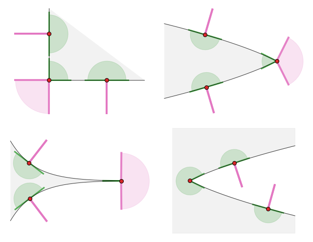
The figure below shows the normal cone (pink area) and the tangent cone (geen area) at several points on the boundary of various sets. Note that the tangent cone includes both the tangent and the feasible directions. The latter are important to clarify the “correct side” of the normal cone, which is always oriented toward the exterior of the set.

5.2.3.5. Constraint qualification

It is possible in some cases to analytically express the tangent cone and the normal cone. More specifically, this may happen when the constraint is defined by an equality or an inequality, such as

\[\begin{split} \mathcal{C}_{\rm level} = \big\{ {\bf w} \in \mathbb{R}^{N} \;|\; h({\bf w}) = 0 \big\}, \\ \mathcal{C}_{\rm sub} = \big\{ {\bf w} \in \mathbb{R}^{N} \;|\; f({\bf w}) \le 0 \big\}. \end{split}\]

In the points where the functions \(f\) and \(h\) are differentiable, one can prove (under reasonable assumptions) that

\[\begin{split} \mathcal{T}_{\mathcal{C}_{\rm level}}({\bf w}) \subseteq \big\{ {\bf t} \in \mathbb{R}^{N} \;|\; {\bf t}^\top \nabla h({\bf w}) = 0 \big\}, \\ \mathcal{T}_{\mathcal{C}_{\rm sub}}({\bf w}) \subseteq \big\{ {\bf t} \in \mathbb{R}^{N} \;|\; {\bf t}^\top \nabla f({\bf w}) \le 0 \big\}. \end{split}\]

The right-hand side is not always equivalent to the tangent cone. When such equivalence holds, we say that the function defining the constraint is qualified. Here are some possible alternatives for constraint qualification.

• \(h({\bf w})\) is affine

• \(f({\bf w})\) is convex and there exists \(\bar{\bf w}\) such that \(f(\bar{\bf w}) <0\)

• \(\nabla h({\bf w})\ne{\bf 0}\) for every \({\bf w}\) such that \(h({\bf w})=0\)

• \(\nabla f({\bf w})\ne{\bf 0}\) for every \({\bf w}\) such that \(f({\bf w})=0\)

Note

If non-zero, the vector \(\nabla \varphi({\bf w})\) is always orthogonal to the curve defined by \(\varphi({\bf w})=0\).

When the functions \(f\) and \(h\) are qualified, the gradients \(\nabla f({\bf w})\) and \(\nabla h({\bf w})\) are always orthogonal to the boundary of the respective constraint sets. Therefore, the normal cones can be analytically expressed as

\[\begin{split} \begin{aligned} (\forall {\bf w}\in\mathcal{C}_{\rm level})\qquad \mathcal{N}_{\mathcal{C}_{\rm level}}({\bf w}) &= \big\{ \lambda \nabla h({\bf w}) \;|\; \lambda\in\mathbb{R} \big\}, \\ (\forall {\bf w}\in\mathcal{C}_{\rm sub})\;\qquad \mathcal{N}_{\mathcal{C}_{\rm sub}}({\bf w}) &= \big\{ \mu \nabla f({\bf w}) \;|\; \mu \ge 0,\; \mu f({\bf w}) = 0 \big\}. \end{aligned} \end{split}\]

This geometrical insight is at the foundation of Lagrange multipliers, because the following holds.

\[\begin{split} \begin{cases} \;\;{\bf w}\in\mathcal{C}_{\rm level} \\ -{\bf d}\in\mathcal{N}_{\mathcal{C}_{\rm level}}({\bf w}) \end{cases} \qquad\iff\qquad (\exists\lambda^*\in\mathbb{R})\; \begin{cases} h({\bf w}) = 0 \\ {\bf d} + \lambda^* \nabla h({\bf w}) = {\bf 0} \end{cases} \\[2em] \begin{cases} \;\;{\bf w}\in\mathcal{C}_{\rm sub} \\ -{\bf d}\in\mathcal{N}_{\mathcal{C}_{\rm sub}}({\bf w}) \end{cases} \qquad\iff\qquad (\exists\mu^*\ge0)\; \begin{cases} f({\bf w}) \le 0 \\ {\bf d} + \mu^* \nabla f({\bf w}) = {\bf 0} \\ \mu^* f({\bf w}) = 0 \end{cases} \end{split}\]

---

[1] (1,2)

The terms “direction” and “vector” are interchangeable. Specifically, “direction” is used to emphasize the idea of a vector that can be expressed as a difference of two other vectors. Geometrically speaking, the direction \({\bf d} = {\bf p} - {\bf w}\) is a vector that originates at \({\bf w}\) and points at \({\bf p}\). But you do not really care about \({\bf p}\) or \({\bf w}\): only the direction \({\bf d}\) is what matters, and it is centered at zero.

[2]

The normal cone at a point \({\bf w}\) is plotted so that it appears to be centered at \({\bf w}\). In reality, normal cone always originates at \({\bf 0}\), but it is shifted in the pictures to facilitate the interpretation.