4.1. Differentiable functions

Differentiable functions play a very important role in optimization. This is because they are locally well approximated as linear functions, so that the notion of derivative suffices to describe their local behavoir. The goal of this introductory section is to discuss some fundamental concepts related to the geometric nature of differentiable functions and their Taylor approximations, in preparation for discussing the gradient descent algorithm.

4.1.1. First derivative

The derivative of a one-dimensional function \(J\colon\mathbb{R}\to\mathbb{R}\) is the rate at which the function changes with respect to an infinitesimal change of its variable. This is formally defined as the limit value of the ratio between such variations

\[ J'(w) = \lim_{h\to0}\frac{J(w+h) - J(w)}{h}. \]

A function is said to be differentiable at a point \(\bar{w}\) if the above limit exists at \(\bar{w}\). Geometrically, this happens when the graph of the function has a unique non-vertical tangent line at the point \((\bar{w}, J(\bar{w}))\). The derivative is precisely the slope of the tangent line at that point. Let’s explore this idea in pictures. The figure below shows the derivative of the function \(J(w)=w^2\) by visually representing the tangent line at each point. Notice how the tangent line hugs the function at every point. This is true in general: the slope of the tangent line always gives local steepness of the function itself. In other words, the tangent line at a point \(\bar{w}\) is the best linear approximation of the function at that point.

First-order approximation (one-dimensional case)

\[ (\forall w\;{\rm near}\;\bar{w})\qquad J(w) \approx J(\bar{w}) + J'(\bar{w}) (w-\bar{w}) \]

The derivative generalizes to a multi-dimensional function \(J\colon\mathbb{R}^N\to\mathbb{R}\) through the notion of partial derivatives. The idea is to calculate the derivative with respect to each coordinate of the function, while helding the others constant. These partial derivatives are then stacked into a vector called the gradient

\[\begin{split} \nabla J({\bf w}) = \begin{bmatrix} \dfrac{\partial J({\bf w})}{\partial w_1}\\ \vdots\\ \dfrac{\partial J({\bf w})}{\partial w_N} \end{bmatrix}. \end{split}\]

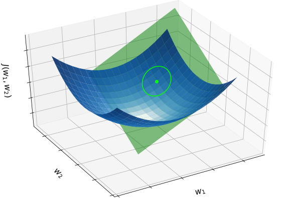
A function is said to be differentiable at a point \({\bf \bar{w}}\) if the partial derivatives exist in a neighborhood of \({\bf \bar{w}}\) and are continuous at \({\bf \bar{w}}\). Geometrically, the gradient at \({\bf \bar{w}}\) defines the slopes of the tangent hyperplane at \(({\bf \bar{w}}, J({\bf \bar{w}}))\), which represents the best linear approximation of the function at \({\bf \bar{w}}\). The figure below shows the quadratic function (blue surface), along with the tangent plane (green surface) defined by the gradient at a point.

First-order approximation (multi-dimensional case)

\[ (\forall {\bf w}\;{\rm near}\;{\bf \bar{w}})\qquad J({\bf w}) \approx J({\bf \bar{w}}) + \nabla J({\bf \bar{w}})^\top ({\bf w}-{\bf \bar{w}}) \]

4.1.2. Second derivative

The second derivative of a one-dimensional function \(J\colon\mathbb{R}\to\mathbb{R}\) measures how the change rate of the function is itself changing. This is formally defined as the derivative of the derivative, namely

\[ J''(w) = \lim_{h\to0}\frac{J'(w+h) - J'(w)}{h}. \]

A function is said to be twice differentiable at a point \(\bar{w}\) if both the first and second derivatives exist at \(\bar{w}\). Geometrically, the second derivative corresponds to the curvature of a function. A function whose second derivative is positive will be curved upwardly (also referred to as convex), meaning that the tangent line will lie below the graph of the function. Similarly, a function whose second derivative is negative will be curved downwardly (also simply called concave), and its tangent lines will lie above the graph of the function. If the second derivative of a function changes sign, the graph of the function will switch from convex to concave, or vice versa. A point where this occurs is called an inflection point.

Just as the first derivative is related to the best linear approximation, the second derivative is related to the best quadratic approximation for a function \(J(w)\). This is the second-order Taylor polynomial of \(J(w)\) centered at point \(\bar{w}\), whose first and second derivatives are precisely \(J'(\bar{w})\) and \(J''(\bar{w})\). Let’s explore this idea in pictures. The figure below shows the second derivative of the function \(J(w)=\sin(2w) + 0.5w^2\) by visually representing the quadratic Taylor polynomial (blue curve) at each point. Notice how it does a much better job at matching the underlying function (black curve) around the center point (red dot) than the tangent line (green curve). Furthermore, the second-order approximation bends up or down according to the curvature of the underlying function at the center point.

Second-order approximation (one-dimensional case)

\[ (\forall w\;{\rm near}\;\bar{w})\qquad J(w) \approx J(\bar{w}) + J'(\bar{w}) (w-\bar{w}) + \frac{1}{2} J''(\bar{w}) (w-\bar{w})^2 \]

The second derivative generalizes to a multi-dimensional function \(J\colon\mathbb{R}^N\to\mathbb{R}\) through the high-order partial derivatives. These include the second-order partials and the mixed partials, arranged into a symmetric matrix known as the Hessian

\[\begin{split} \nabla^2 J({\bf w}) = \begin{bmatrix} \dfrac{\partial^2 J({\bf w})}{\partial w_1 \partial w_1} & \dots & \dfrac{\partial^2 J({\bf w})}{\partial w_1 \partial w_N}\\ \vdots & \ddots & \vdots \\ \dfrac{\partial^2 J({\bf w})}{\partial w_N \partial w_1} & \dots & \dfrac{\partial^2 J({\bf w})}{\partial w_N \partial w_N} \end{bmatrix}. \end{split}\]

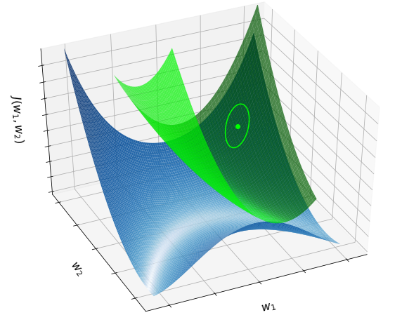
The eigenvalues of this matrix reveal the convexity/concavity of a function. More specifically, a function at a point \({\bf \bar{w}}\) is convex along its \(n\)-th coordinate (while helding the others constant) if and only if the \(n\)-th eigenvalue of its Hessian at \({\bf \bar{w}}\) is non-negative. It is jointy convex if and only if all the eigenvalues are non-negative. In complete analogy to the one-dimensional case, the Hessian is related to the best quadratic approximation of the function at a given point. The figure below shows the Rosenbrock function (blue surface), along with the quadratic approximation (green surface) at a point.

Second-order approximation (multi-dimensional case)

\[ (\forall {\bf w}\;{\rm near}\;{\bf \bar{w}})\qquad J({\bf w}) \approx J({\bf \bar{w}}) + \nabla J({\bf \bar{w}})^\top ({\bf w}-{\bf \bar{w}}) +\frac{1}{2} ({\bf w}-{\bf \bar{w}})^\top \nabla^2 J({\bf \bar{w}}) ({\bf w}-{\bf \bar{w}})\]

4.1.3. Differentiability classes

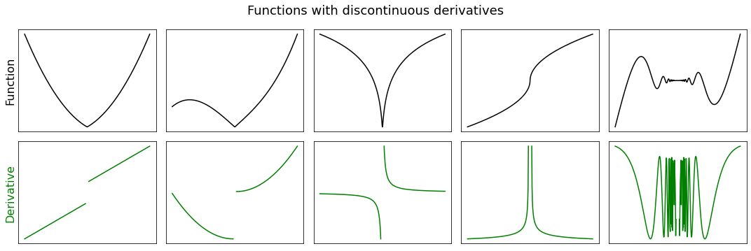
Most functions that occur in practice have derivatives at all points or at almost every point. If a function is differentiable at a point, then it must also be continuous at that point. The converse does not hold, in the sense that a continuous function needs not be differentiable everywhere. The classical example is a continuous function with a corner, a cusp, or a vertical tangent, which fails to be differentiable at the location of the anomaly. Moreover, not all differentiable functions have continuous derivatives, like for example the function \(f(x) = x^2\sin(1/x)\), whose derivative \(f'(x)=2x\sin(1/x) - \cos(1/x)\) exists everywhere but it is discontinuous at \(x=0\) since \(f'(0)=0\). Discontinuous derivatives may cause issues in the context of optimization. This is why there exist different levels of differentiability with stronger and stronger requirements.

• Differentiable almost everywhere: A function that is differentiable at all points except a subset of measure zero. This is a continuous function with isolated singularities, such as corners, cusps, vertical tangents, or discontinuities. The derivative has a discontinuity at the location of the anomaly.

• Differentiable (everywhere): A function that is differentiable at every point of its domain. This is a continuous function with no singularity, except for a possible removable discontinuity. The derivative never has a jump discontinuity, but it may have an essential discontinuity at the location of the possible anomaly.

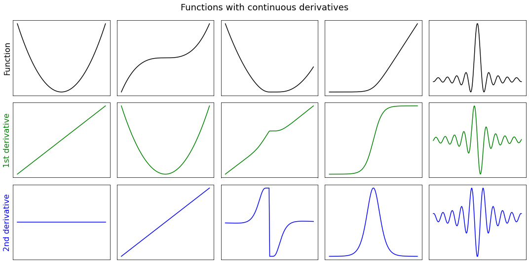
• Continuously differentiable: A differentiable function with a continuous derivative. As such, the derivative cannot change too fast locally (but could globally). If a differentiable function is convex, then it is continuously differentiable.

• Lipschitz differentiable: A function with a continuous derivative that is globally limited in how fast it can change. This is a function whose curvature is bounded, namely the second derivative is upper bounded by a constant.

The following facts relate the different classes of differentiability.

• Lipschitz differentiable \(\Rightarrow\) Continuously differentiable \(\Rightarrow\) Differentiable \(\Rightarrow\) Differentiable almost everywhere.

• Twice differentiable \(\implies\) Continuously differentiable.

• Twice differentiable + Bounded second derivatives \(\implies\) Lipschitz differentiable.

• Lipschitz differentiable \(\implies\) Twice differentiable almost everywhere.

• Convex and differentiable \(\implies\) Continuously differentiable.

From now on, it will be always required that a function is Lipschitz differentiable, or at least continuously differentiable. Many first-order optimization algorithms rely on this assumption, including the gradient descent method. They rarely work without any precaution if the function has a weaker type of differentiability. Nonetheless, several “fixes” have been specifically designed to deal with almost-everywhere differentiable functions (and even with non-differentiable functions). They are however outside the scope of this chapter.

Blanket assumption

The cost function \(J({\bf w})\) is Lipschitz differentiable (or at least continuously differentiable).

4.1.4. Smooth convexity

If a function is twice differentiable, then the following holds.

• Convexity requires the second derivatives to be non-negative.

• Strict convexity requires the second derivatives to be positive, although they can get arbitrarily small.

• Strong convexity requires the second derivatives to be lower bounded by a positive value \(\mu>0\).

More precisely, the Hessian matrix of a twice-differentiable function \(J({\bf w})\) is related to convexity as follows.

\[\begin{split} \begin{aligned} \nabla^2 J({\bf w}) \ge 0 &\quad\Rightarrow\quad \textrm{convex} \\ \nabla^2 J({\bf w}) > 0 &\quad\Rightarrow\quad \textrm{strictly convex} \\ \nabla^2 J({\bf w}) \ge \mu I > 0 &\quad\Rightarrow\quad \textrm{strongly convex} \end{aligned} \end{split}\]