5.4.2. Affine space

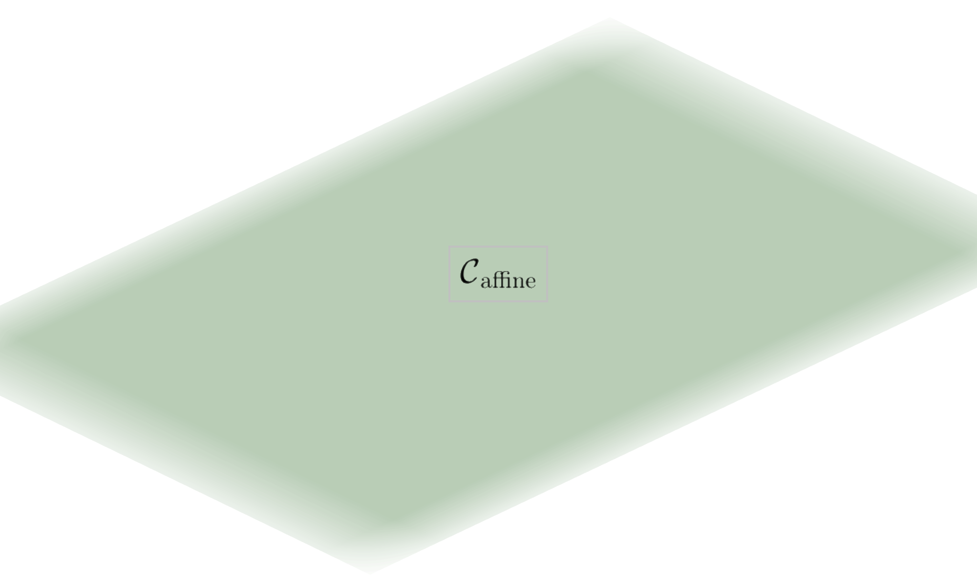
For a given matrix \(A \in \mathbb{R}^{K \times N}\) and vector \({\bf b} \in \mathbb{R}^K\), the affine space is a linear constraint defined as

\[ \mathcal{C}_{\rm affine} = \big\{ {\bf w} \in \mathbb{R}^{N} \;|\; A {\bf w} = {\bf b} \big\}. \]

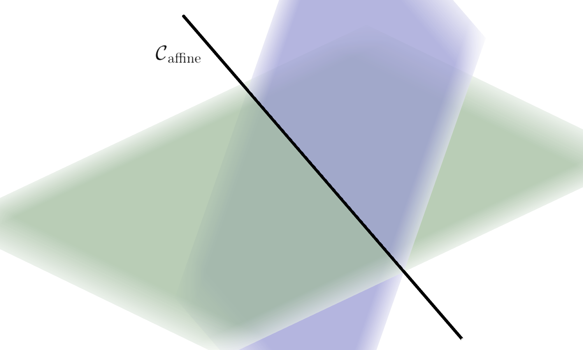
The conditions \(K \le N\), \({\rm rank}(A)=K\), and \({\bf b}\in{\rm ran}(A)\) are required for this subset to be nonempty. Simply put, \(A\) must have linearly independent rows, and \({\bf b}\) must belong to its column space. Note that an affine space may or may not be a vector space, depending on whether it contains the zero vector. The figure below shows several affine constraints in \(\mathbb{R}^{3}\).

Affine space with \(N=3\) and \(K=1\)

Affine space with \(N=3\) and \(K=2\)

5.4.2.1. Constrained optimization

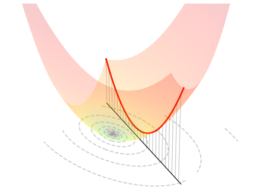
Optimizing a function \(J({\bf w})\) over an affine space can be expressed as

\[ \operatorname*{minimize}_{\textbf{w}\in\mathbb{R}^N}\;\; J({\bf w}) \quad{\rm s.t.}\quad A {\bf w} = {\bf b}. \]

The figure below visualizes such an optimization problem in \(\mathbb{R}^{2}\).

5.4.2.2. Orthogonal projection

The projection of a point \({\bf u}\in\mathbb{R}^{N}\) onto the affine space is the (unique) solution to the problem

\[ \operatorname*{minimize}_{{\bf w}\in\mathbb{R}^N}\;\; \|{\bf w}-{\bf u}\|^2 \quad{\rm s.t.}\quad A {\bf w} = {\bf b} \]

The solution can be analytically computed as follows.

Projection onto the affine space

\[ \mathcal{P}_{\mathcal{C}_{\rm affine}}({\bf u}) = {\bf u} - A^\top(A A^\top)^{−1}(A {\bf u} - {\bf b}) \]

5.4.2.3. Implementation

The python implementation is given below.

def project_affine(u, A, b):
    
    assert np.linalg.matrix_rank(A) == A.shape[0], "The matrix must have full row rank"
    
    s = np.linalg.solve(A @ A.T, A @ u - b)
    p = u - A.T @ s
    
    return p

Here is an example of use.

u = np.array([-1, 2, 4])

A = np.array([[1, -1,  0],
              [0,  1, -1]])

b = np.array([1, -1])

p = project_affine(u, A, b)

5.4.2.4. Proof

By using the Lagrange multipliers to remove the equality constraint, the projection onto the affine space is the (unique) solution to the following problem

\[ \operatorname*{minimize}_{{\bf w}\in\mathbb{R}^N}\;\sup_{{\bf c}\in\mathbb{R}^K}\; \frac{1}{2}\|{\bf w}-{\bf u}\|^2 + {\bf c}^\top (A {\bf w} - {\bf b}). \]

Strong duality holds, because this is a convex problem with linear constraints. Hence, it can be equivalently rewritten as

\[ \operatorname*{maximize}_{{\bf c}\in\mathbb{R}^K}\;\inf_{{\bf w}\in\mathbb{R}^N}\; \frac{1}{2}\|{\bf w}-{\bf u}\|^2 + {\bf c}^\top (A {\bf w} - {\bf b}). \]

Setting to zero the gradient w.r.t. \({\bf w}\), the inner minimization is solved by

\[ {\bf w}^* = {\bf u} - A^\top {\bf c}. \]

Setting to zero the gradient w.r.t. \({\bf c}\), the outer maximization is attained by the vector \({\bf c}\) that solves the equation

\[ A {\bf w}^* = {\bf b} \quad\Leftrightarrow\quad A {\bf u} - AA^\top {\bf c} = {\bf b} \quad\Leftrightarrow\quad {\bf c} = (AA^\top)^{-1}(A {\bf u} - {\bf b}) . \]