4.4. Gradient descent

Local optimization aims at finding a minimum of a function \(J({\bf w})\) through an iterative process that starts at some point \({\bf w}_0\) and proceeds by generating a sequence of points \({\bf w}_{k+1} = {\bf w}_k + {\bf d}_k\) for \(k=0,1,\dots,K\). Here, the vector \(\mathbf{d}_k\) is assumed to be a descent direction that leads to a point \(\mathbf{w}_{k+1}\) lower than \(\mathbf{w}_{k}\) on the function, so that \(J(\mathbf{w}_{k+1}) < J(\mathbf{w}_{k})\). One of the most efficient way to compute a high-quality descent direction is to leverage the negative gradient of \(J({\bf w})\), leading to the optimization algorithm known as gradient descent or gradient method.

4.4.1. Descent direction

The derivative of a one-dimensional function describes its tangent lines. It thus gives a precise indication of where the nearest minimum is located with respect to a given point. For example, if the derivative at a point \(w_k\) is negative, one should “go right” to find a point \(w_{k+1}\) that is lower on the function. Conversely, if the derivative at \(w_k\) is positive, one should “go left” to lower the function. This fact is shown in the next figure for the function \(J(w)=\sin(3w)+\frac{1}{2}w^2\), where the negative derivative \(-J'(w)\) is plotted as a vector in red along the horizontal axis. By moving the slider from left to right, one can observe that the negative derivative always indicates the direction where the function decreases, although only “locally”.

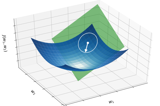
Precisely the same idea holds for a high-dimensional function \(J({\bf w})\), only now there is a multitude of partial derivatives. When combined into the gradient, they indicate the direction and rate of fastest increase for the function at each point. This means that the negative gradient at a point indicates the direction in which the function decreases most quickly from that point. The next figure illustrates this fact for the quadratic function \(J({\bf w}) = \|{\bf w}\|^2\), where the negative gradient (white arrow) at a given point (white dot) provides the direction that decreases the function locally.

4.4.2. Algorithm

Gradient descent is a local optimization algorithm that employs the negative gradient as a descent direction at each iteration. Given an initial point \({\bf w}_0\) and a step size \(\alpha>0\), the generic update step is written as follows.

Gradient descent

\[ {\bf w}_{k+1} = {\bf w}_k - \alpha\nabla J({\bf w}_k) \]

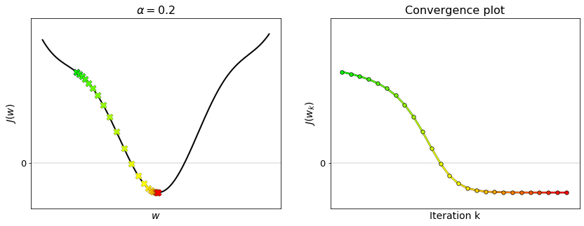
This iterative scheme is illustrated in the figure below for a one-dimensional function. Moving the slider from left to right animates each step of gradient descent. At each iteration, the next point (red dot) is generated based on the derivative (green line) at the current point (pink dot). The tangent line flattens more and more as the current point converges to the minimum. This is because the derivative is continuous, and thus it gradually shrinks to zero when approaching a minimum.

The basic intuition behind gradient descent can be illustrated by a hypothetical scenario. A person is stuck in the mountains and is trying to get down. There is heavy fog such that visibility is extremely low. Since the path down the mountain is not visible, they are forced to resort only to clues in their proximity to find the way down. They can use the method of gradient descent, which involves looking at the steepness of the hill at their current position, then proceeding downhill in the direction with the steepest descent. Using this method, they would eventually find their way down the mountain or possibly get stuck in some plateau, like a mountain lake. However, assume also that the steepness of the hill is not immediately obvious with simple observation, but rather it requires a sophisticated instrument to measure, which the person happens to have at the moment. It takes quite some time to measure the steepness of the hill with the instrument, thus they should minimize their use of the instrument if they wanted to get down the mountain before sunset. The difficulty then is choosing the frequency at which they should measure the steepness of the hill so not to go off track.

In this analogy, the person represents the algorithm, and the path taken down the mountain represents the sequence of points that the algorithm will explore. The steepness of the hill represents the slope of a cost function at that point. The instrument used to measure steepness is differentiation. The direction they choose to follow is the gradient at that point. The distance they travel before taking another measurement is the step-size. Source: wikipedia

4.4.3. Step-size

The gradient method comes equipped with the step-size. This is a positive value \(\alpha>0\) that controls the distance travelled along the negative gradient direction at each iteration. Indeed, it can be easily proved that the distance between two consecutive iterates \({\bf w}_k\) and \({\bf w}_{k+1}\) is equal to the gradient magnitude scaled by the step-size:

\[ \| {\bf w}_{k+1} - {\bf w}_k \| = \| {\bf w}_k - \alpha\nabla J({\bf w}_k) - {\bf w}_k \| = \alpha \| \nabla J({\bf w}_k) \|. \]

If the step-size \(\alpha\) is chosen sufficiently small, the algorithm will stop at a stationary point of the function \(J({\bf w})\). This arises by the very form of gradient descent itself. Indeed, when the new point \({\bf w}_{k+1}\) does not move significantly from \({\bf w}_k\), it can only mean that the gradient is vanishing, namely that \(\nabla J({\bf w}_k)\approx {\bf 0}\). This is by definition a stationary point of the function \(J({\bf w})\).

4.4.4. Convergence plot

A useful way to analyze the progress of gradient descent is to evaluate the cost function at each point \({\bf w}_k\) generated by the algorithm, so as to store the sequence of values

\[ J({\bf w}_0), J({\bf w}_1),\dots, J({\bf w}_k). \]

These values contain the history of a single run of the gradient descent method. Their visualization results in the so-called convergence plot. Such plot is an invaluable debugging tool for gradient descent, especially when dealing with high-dimensional cost functions, since they cannot be visualized in any other way. As a rule of thumb, it is always advised to inspect the convergence plot whenever you run the gradient descent algorithm.

The figure below shows the convergence plot obtained from the previous example. Note that the convergence plot decreases and eventually flattens. This is a good indication that gradient descent converged to a minimum of the function.

4.4.5. Numerical implementation

The following is the Python implementation of gradient descent. Autograd is used for automatic differentiation.

def gradient_descent(cost_fun, init, alpha, epochs):
    """
    Finds a minimum of a function.
    
    Arguments:
    cost_fun -- cost function | callable that takes 'w' and returns 'J(w)'
    init     -- initial point | vector of shape (N,)
    alpha    -- step-size     | positive scalar
    epochs   -- n. iterations | integer
    
    Returns:
    w       -- final point     | vector of shape (N,)
    history -- function values | vector of shape (epochs+1,)
    """
    
    # Automatic gradient
    from autograd import grad 
    gradient = grad(cost_fun)
    
    # Initialization
    w = np.array(init, dtype=float)
    J = cost_fun(w)
    
    # Iterative refinement
    history = [J]
    for k in range(epochs):
        
        # Gradient step
        w = w - alpha * gradient(w)
        
        # Tracking
        history.append(cost_fun(w))
            
    return w, history

The python implementation requires four arguments:

• the function to optimize,

• a starting point,

• a step-size that controls the distance travelled at each iteration,

• the number of iterations to be performed.

An usage example is presented next.

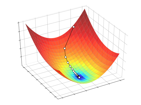
# cost function of two variables
cost_fun = lambda w: (2*w[0]+1)**2 + (w[1]+2)**2

init   = [1., 3.]  # initialization
alpha  = 0.1       # step-size
epochs = 30        # number of iterations
    
# numerical optimization
w, history = gradient_descent(cost_fun, init, alpha, epochs)

The process of optimizing this function with gradient descent is illustrated below.

4.4.6. Appendix: Flattening

The following is a more general implementation of gradient descent. It not only works with arrays, but also with any combination of lists, tuples, or dictionaries. In the latter case, the only requirement is that all the numbers in the “initial point” are converted to the float type, otherwise an error will be trown.

def gradient_descent(cost_fun, init, alpha, epochs):
    """
    Finds a minimum of a function.
    
    Arguments:
    cost_fun -- cost function | callable that takes 'w' and returns 'J(w)'
    init     -- initial point | array, list, tuple, dictionary of float values
    alpha    -- step-size     | scalar
    epochs   -- n. iterations | integer
    
    Returns:
    w       -- final point     | vector of shape (N,)
    history -- function values | vector of shape (epochs+1,)
    """
    from autograd.misc.flatten import flatten
    from autograd import grad
    
    # Flattening
    flat, unflatten = flatten(init)
    flat_cost_fun = lambda w: cost_fun(unflatten(w))
    
    # Automatic gradient
    gradient = grad(flat_cost_fun)
    
    # initialization
    w = np.array(flat, dtype=float)
    J = flat_cost_fun(w)
    
    # gradient descent
    history = [J]
    for k in range(epochs):
        
        # Gradient step
        w = w - alpha * gradient(w)

        # Tracking
        history.append(flat_cost_fun(w))
        
    return unflatten(w), history