5.4.4. Half-space

For a given vector \({\bf c}\in\mathbb{R}^N\) and scalar \(\eta\in\mathbb{R}\), the half-space is a linear constraint defined as

\[ \mathcal{C}_{\rm half} = \big\{ {\bf w} \in \mathbb{R}^{N} \;|\; {\bf c}^\top {\bf w} \le \eta \big\}. \]

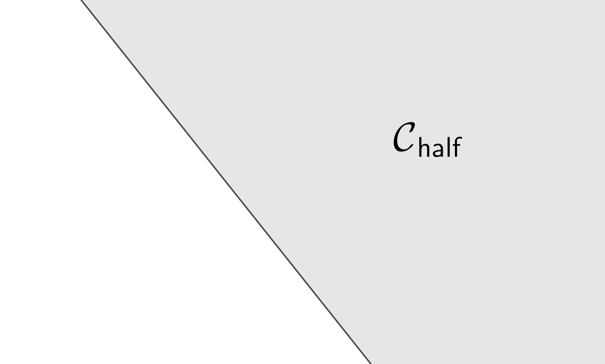
The figure below shows how this constraint looks like in \(\mathbb{R}^{2}\) or in \(\mathbb{R}^{3}\).

Half-space in 2D

Half-space in 3D

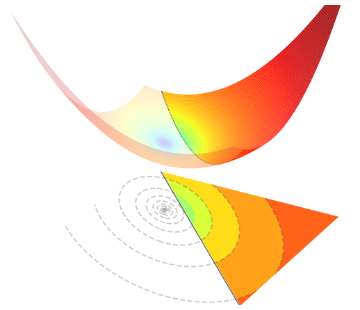
5.4.4.1. Constrained optimization

Optimizing a function \(J({\bf w})\) over an half-space can be expressed as

\[ \operatorname*{minimize}_{\textbf{w}\in\mathbb{R}^N}\;\; J({\bf w}) \quad{\rm s.t.}\quad {\bf c}^\top {\bf w} \le \eta. \]

The figure below visualizes such an optimization problem in \(\mathbb{R}^{2}\).

5.4.4.2. Orthogonal projection

The projection of a point \({\bf u}\in\mathbb{R}^{N}\) onto the half-space is the (unique) solution to the following problem

\[ \operatorname*{minimize}_{{\bf w}\in\mathbb{R}^N}\;\; \|{\bf w}-{\bf u}\|^2 \quad{\rm s.t.}\quad {\bf c}^\top {\bf w} \le \eta. \]

The solution can be analytically computed as follows.

Projection onto the half-space

\[\begin{split} \mathcal{P}_{\mathcal{C}_{\rm half}}({\bf u}) = \begin{cases} {\bf u} &\textrm{if ${\bf c}^\top {\bf u} \le \eta$}\\ {\bf u} + {\bf c} \, \Big(\dfrac{\eta - {\bf c}^\top {\bf u} }{\|{\bf c}\|_2^2}\Big) &\textrm{otherwise} \end{cases} \end{split}\]

5.4.4.3. Implementation

The python implementation is given below.

def project_half(u, coefs, bound):
    
    s = np.minimum(0, bound - np.sum(u * coefs)) / np.sum(coefs**2)
    p = u + s * coefs 
    
    return p

Here is an example of use.

u = np.array([-1, 2, 4])

coefs = np.array([1, 2, 1])
bound = 1

p = project_half(u, coefs, bound)