4.2. Automatic differentiation

The gradient plays a central role in differentiable optimization. For this reason, there are special calculators to automatically compute the gradient of arbitrary complicated mathematical functions, which free us from the burden of having to calculate it on paper. Gradient calculators are commonly called Automatic Differentiators. In this section, we demonstrate how to use the autograd package, a simple yet powerful automatic differentiator written in Python.

4.2.1. Autograd

Autograd can automatically differentiate native Python and Numpy code. It can handle a large subset of Python’s features, including loops, ifs, recursion, and closures. It supports reverse-mode differentiation (a.k.a. backpropagation), which means it can efficiently take gradients of scalar-valued functions with respect to array-valued arguments.

Since autograd is specially designed to automatically compute the derivatives of NumPy code, it comes with its own wrapper on the numpy library. This is where the differentiation rules are defined. We can use autograd’s version of numpy exactly like you would the standard version. The line below is used to import this autograd wrapped version of numpy.

import autograd.numpy as np

Moreover, autograd provides the function grad() to perform the automatic differentiation. The commannd grad() takes in a function that returns a scalar-valued float output, and gives us another function that computes its derivative. This covers the common case of gradients used for optimization.

from autograd import grad

Now, let’s compute a few derivatives using autograd.

4.2.2. Derivative of a (one-dimensional) function

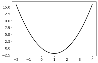
We begin the demonstration with the simple function of one variable

\[ (\forall w\in \mathbb{R})\qquad f(w) = a w^2 - bw, \]

whose derivative is

\[f'(w) = 2a w - b. \]

The common way of defining a function in Python is via the standard def declaration.

def function(w, a, b):
    return a * w**2 - b * w

We can also create inline functions in Python by using the lambda keyword.

function = lambda w, a, b: a * w**2 - b * w

There is no difference between these two ways of defining a function in Python. You can visualize either version of the function using matplotlib. Below the function is plotted over the points \(w\in[−2,4]\), after setting \(a=2\) and \(b=4\).

w_list = np.linspace(-2, 4)

f_list = [function(w, a=2, b=4) for w in w_list]

Now, you can compute the derivative of our function using grad(). When the function presents multiple inputs, the derivative is computed with respect to the first argument. As for the function defined in the above example, the derivative is computed against w, which is what you want. An optional integer parameter can be used to specify the positional argument in respect of which compute the derivative.

derivative = grad(function)

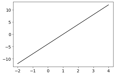
The result of grad() is a Python function that can be used to evaluate the derivative at any point. Below is plotted the derivative over the points \(w\in[−2,4]\) after setting \(a=2\) and \(b=4\). Remark that it corresponds to the analytical expression given earlier.

g_list = [derivative(w, a=2, b=4) for w in w_list]

Notice that derivative() only accepts scalar values, because it implements the derivative of a one-variable function. An error is thrown if an array is passed as input.

w = np.array([0.,0.])
g = derivative(w)

---------------------------------------------------------------------------
TypeError                                 Traceback (most recent call last)
      1 w = np.array([0.,0.])
----> 2 g = derivative(w)

TypeError: Grad only applies to real scalar-output functions. Try jacobian or elementwise_grad.

4.2.3. Gradient of a (multi-dimensional) function

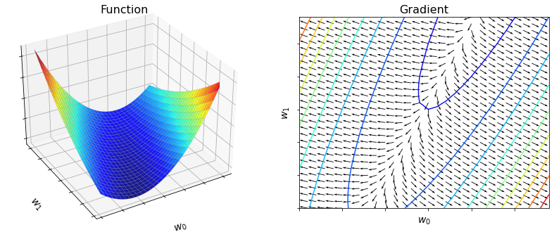
Consider the scalar function of multiple variables

\[ (\forall {\bf w}=[w_0,w_1]^\top\in \mathbb{R}^2)\qquad f({\bf w}) = w_0^2 + (2 w_0 - w_1)^2 - 2w_1, \]

whose gradient is the vectorial function of multiple variables

\[\begin{split} \nabla f({\bf w}) = \begin{bmatrix} \frac{\partial f}{\partial w_0}\\ \frac{\partial f}{\partial w_1}\\ \end{bmatrix} = \begin{bmatrix} 10 w_0 - 4 w_1\\ -4 w_0 + 2 w_1 - 2 \end{bmatrix}. \end{split}\]

To compute the gradient with autograd, you are required to write a function in which the first argument is a NumPy array gathering all the variables in respect of which compute the gradient. In other words, rather than defining the above \(f({\bf w})\) as a Python function with two separate inputs, you should define a function taking a single NumPy array as the first positional argument. You can then use indexing and slicing to access the array elements.

def function(w):
    w = np.array(w, dtype=float)  # NumPy array of float numbers!
    return w[0]**2 + (2 * w[0] - w[1])**2 - 2 * w[1]

Now, it is straighforward to compute the gradient using grad().

gradient = grad(function)

Below the function and the gradient are plotted over a grid of points.

span = np.arange(-3, 3, 0.2)
X, Y = np.meshgrid(span, span)
w_list = np.stack([X.ravel(), Y.ravel()], axis=1)

f_list = [function(w) for w in w_list]
g_list = [gradient(w) for w in w_list]

4.2.4. Supported parts of NumPy

Not all the NumPy features can be used with autograd. For example, autograd supports indexing (x = A[i, j, :]) but not assignment (A[i,j] = x) in arrays that are being differentiated with respect to. Assignment is hard to support because it requires keeping copies of the overwritten data, and so even when you write code that looks like it’s performing assignment, the system would have to be making copies behind the scenes, often defeating the purpose of in-place operations. Here is an overview of what you can do in autograd, and what you should avoid instead.

Do use

• Most of numpy’s functions

• Most np.array methods

• Some scipy functions

• Indexing and slicing of arrays x = A[3, :, 2:4]

• Explicit array creation from lists A = np.array([x, y]).

Don’t use

• Assignment to arrays A[0,0] = x

  • Create new arrays through vectorized operations instead!

• Creation of lists w = [x, y]

  • Use w = np.array([x, y]) instead!

• Implicit casting of lists to arrays A = np.sum([x, y])

  • Use A = np.sum(np.array([x, y])) instead!

• In-place operations such as a += b

  • Use a = a + b instead!

• The operation A.dot(B)

  • Use np.dot(A, B) or A @ B instead!

4.2.5. Appendix: Flattening of a function

This short section discusses a useful pre-processing technique called function flattening, which allows you to express any mathematical function in the generic form \(J({\bf w})\) that has been using thus far. For example, consider the following function

\[ \psi(a, {\bf b}, C) = \left(a + {\bf 1}^\top {\bf b} + {\bf 1}^\top C {\bf 1}\right)^2 \]

where \(a \in \mathbb{R}\) is a scalar, \({\bf b} \in \mathbb{R}^3\) is a vector, and \(C \in \mathbb{R}^{3\times 3}\) is a matrix, with \({\bf 1} = [1,\dots,1]^\top\) being the vector of all ones. This function is not written in the generic form \(J({\bf w})\). There is a absolutely nothing wrong with it. However, autograd requires that \(\psi(a, {\bf b}, C)\) is implemented as a python function taking a single numpy array as input. To accomodate this requirement, we must flatten and concatenate the variables \(a, {\bf b}, C\) into a single contiguous vector \({\bf w}\), as follows

\[\begin{split} {\bf w} = \begin{bmatrix} w_1 \\ w_2 \\ w_3 \\ w_4 \\ w_5 \\ \vdots \\ w_{13} \\ \end{bmatrix} = \begin{bmatrix} a \\ b_1 \\ b_2 \\ b_3 \\ C_{1,1} \\ \vdots \\ C_{3,3}\\ \end{bmatrix}. \end{split}\]

Now, the function \(\psi(a, {\bf b}, C)\) can be equivalently rewritten as

\[ J({\bf w}) = \left({\bf 1}^\top {\bf w}\right)^2. \]

The process of flattening a cost function can be performed automatically with the routine flatten_func() imported from the autograd library.

from autograd.misc.flatten import flatten_func

Here is how you can automatically flatten the cost function \(\psi(a, {\bf b}, C)\). First, gather all the input variables in a Python collection such as a tuple, a list, or a dictionary.

a = 1.
b = 2*np.ones(3)
c = 3*np.ones((3,3))

w_tuple = (a, b, c)

--- Original parameters ---
a: 1.0
b: [2. 2. 2.]
c: [[3. 3. 3.]
    [3. 3. 3.]
    [3. 3. 3.]]

Then, implement the “original” cost function \(\psi(a, {\bf b}, C)\) through a python function taking the tuple as input. The tuple is then unpacked inside the function.

def original_cost(w_tuple):
    a, b, c = w_tuple
    z = np.ones(3)
    return (a + z @ b + z @ c @ z)**2

c = original_cost(w_tuple)

Finally, create the “flatten” cost function \(J({\bf w})\) by invoking flatten_func().

flatten_cost, unflatten_func, w_flat = flatten_func(original_cost, w_tuple)

--- Flatten parameters ---
w_flat: [1. 2. 2. 2. 3. 3. 3. 3. 3. 3. 3. 3. 3.]

Now, we can easily compute the gradient of \(J({\bf w})\) using grad().

flatten_gradient = grad(flatten_cost)

g = flatten_gradient(w_flat)

In the next section, you will integrate this technique directly into the code implementing gradient descent, so that you will never have to worry about the issues related to function flattening.