5.7.3. Example 8

Portfolio optimization is a mathematical framework for building a portfolio of assets such that the combined expected return is maximized for a given level of risk. It formalises the notion of diversification, which is the idea that investing in different kinds of financial assets is less risky than owning only one type. This approach was invented by Harry Markowitz in 1952.

5.7.3.1. Candidate assets

Let us create an hypothetical portfolio with 6 candidate assets. We are going to use the stocks of popular American technology companies, such as Facebook, Amazon, Apple, Netflix, Alphabet, Tesla. Building an optimal portfolio requires knowledge of the expected return and the financial risk for each candidate asset. This is what we are going to do next.

5.7.3.1.1. Historical stock prices

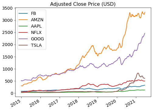
First of all, we fetch the “adjusted close” price of each asset from 2015 to today. This is done in the following code snippet.

import pandas as pd
from datetime import datetime
from pandas_datareader import data as web

# candidate assets
assets = ["FB", "AMZN", "AAPL", "NFLX", "GOOG", "TSLA"]

# temporal window
start = '2015-01-01'
today = datetime.today().strftime('%Y-%m-%d')

# Store the "Adjusted Close" price of each stock into a data frame
price = pd.DataFrame()
for stock in assets:
    price[stock] = web.DataReader(stock, data_source='yahoo', start=start, end=today)['Adj Close']

The figure below shows the historical prices of the candidate assets.

5.7.3.1.2. Annualized expected returns

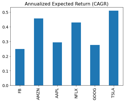
Portfolio optimization requires to know the expected return of each asset considered for inclusion in the portfolio. The expected return of an asset is the percentage change in the asset price over a standard year of 252 trading days. In practice, the expected return is rather difficult to forecast with any certainty. The best we can do is to come up with an estimate, for example by extrapolating historical data.

The simplest estimate of the expected return is the mean value of the percentage change in the asset price. Assuming the daily prices are given as the sequence \(a_0, a_1,\dots, a_N\) of length \(N+1\), the growth rate on a given day \(k\) is the ratio \(a_{k}/a_{k-1}\). The geometric mean of the daily growth rate is thus equal to \(\sqrt[N]{\frac{a_1}{a_0} \frac{a_2}{a_1} \cdots \frac{a_N}{a_{N-1}}} = \sqrt[N]{\frac{a_N}{a_0}}\). Such number is then raised to the power of 252 and subtracted by 1 to obtain the annualized percentage change:

\[ \textsf{Expected Return} = \left(\frac{a_N}{a_0}\right)^\frac{252}{N} - 1. \]

This formula is also known as the compound annual growth rate. The exponent 252 accounts for the fact that we have daily prices, whereas a standard year is made of 252 trading days. In other terms, we compute the mean value of the daily growth rate, and then we assume that such rate occurs identically for all 252 days in a standard year. The exponent 255 should be replaced by 12 if we had montly prices, or by 1 if we had annual prices.

frequency = 252  # Number of trading days in a standard year

length = price.count() - 1  # Number of days (minus one) in the data

expected_return = (price.iloc[-1] / price.iloc[0]) ** (frequency / length) - 1

The figure below shows the historical estimation of the expected return for each candidate asset.

Warning

Estimating the expected return is a critical step in portfolio optimization. Various methods exist to tackle such task, each with its advantages and drawbacks. If predicting stock returns were as easy as calculating the mean historical return, we would all be rich!

5.7.3.1.3. Annualized risk

The risk is the potential financial loss stemming from an investment. The most common way to quantify the risk of a portfolio is through the covariance matrix, which describes the volatility of candidate assets and how they correlate with one another. This information is important because risk can be reduced by investing in many uncorrelated assets. The problem however is that we do not have access to the covariance matrix. The only thing we can do is to make estimates based on past data.

To estimate the covariance matrix, we must convert the historical asset prices into daily percentage returns. These are nothing but the daily percentage changes in the asset price, which can be computed through the following formula:

\[ \textsf{Daily Return} = \frac{\textsf{Today's Price}}{\textsf{Yesterday's Price}} - 1. \]

Then, we compute the sample covariance matrix of the daily returns, and we multiply the result by 252 to obtain the annualized estimation. Note that a diagonal entry of the sample covariance matrix is the variance of an asset, whereas an off-diagonal entry is the covariance between a pair of assets.

daily_return = price.pct_change().dropna()

risk_matrix = daily_return.cov() * 252

The table below shows the estimated covariance matrix of the candidate assets.

	FB	AMZN	AAPL	NFLX	GOOG	TSLA
FB	0.101	0.058	0.054	0.060	0.057	0.060
AMZN	0.058	0.093	0.050	0.068	0.053	0.062
AAPL	0.054	0.050	0.087	0.052	0.048	0.064
NFLX	0.060	0.068	0.052	0.178	0.055	0.075
GOOG	0.057	0.053	0.048	0.055	0.073	0.053
TSLA	0.060	0.062	0.064	0.075	0.053	0.310

Warning

Although the most straightforward approach is to just calculate the sample covariance matrix based on historical returns, recent studies indicate that there exist much more robust statistical estimators of the covariance matrix. The sample covariance matrix should not be your default choice when real money is at stake!

5.7.3.2. Portfolio optimization

A portfolio can be represented as a vector that expresses the fraction of investment on each candidate asset.

\[\begin{split} {\bf w} = \begin{bmatrix} w_1\\ w_2\\ w_3\\ w_4\\ w_5\\ w_6 \end{bmatrix} \begin{aligned} &\to {\sf FB}\\ &\to {\sf AMZN}\\ &\to {\sf AAPL}\\ &\to {\sf NFLX}\\ &\to {\sf GOOG}\\ &\to {\sf TSLA} \end{aligned} \end{split}\]

For example, a portfolio that invests 20% of the available capital in FB stocks, 40% in AMZN, 30% in AAPL, and 10% in TSLA is represented by the vector \({\bf w} = [0.2, 0.4, 0.3, 0, 0, 0.1]^\top\), whereas a portfolio that equally diversifies the investment over all the stocks is given by \({\bf w} = [1/6, 1/6, 1/6, 1/6, 1/6, 1/6]^\top\). This representation leads to the following indicators.

• Portfolio return: The combined return of all the assets being included in a portfolio. Assuming the vector \({\bf r}\) holds the expected returns of all the candidate assets, this is equal to

\[ \textsf{Return}({\bf w}) = {\bf r}^\top {\bf w} = \sum_i r_i w_i. \]

• Portfolio risk: The combined risk of all the assets being included in a portfolio. Given the covariance matrix \(C\) of all the candidate assets, this is equal to

\[ \textsf{Risk}({\bf w}) = {\bf w}^\top C {\bf w} = \|C^{\frac{1}{2}} {\bf w}\|^2 = \sum_i\sum_j c_{ij} w_i w_j. \]

5.7.3.2.1. Mean-Variance tradeoff

Even with a limited number of assets, the composition of a portfolio involves an infinite number of possibilities. Portfolio optimization aims at finding a composition that allows the investor to achieve the highest return for a given amount of risk. This can be equivalently translated into the minimization of the financial risk minus the expected return multiplied by a risk-tolerance parameter, under the constraint that all the capital must be invested in the portfolio. Such considerations lead to the constrained optimization problem formulated as follows:

\[\begin{split} \operatorname*{minimize}_{{\bf w}\in\mathbb{R}^N}\quad {\bf w}^\top C {\bf w} - \gamma \, {\bf r}^\top {\bf w} \quad\textrm{subject to}\quad \begin{cases} {\bf w} \ge 0 \\ {\bf 1}^\top {\bf w} = 1. \end{cases} \end{split}\]

Note that the parameter \(\gamma\ge0\) specifies the “risk tolerance” for the desired portfolio.

• The choice \(\gamma=0\) results in the portfolio with minimal risk.

• The choice \(\gamma\to+\infty\) leads to riskier but more profitable portfolios.

5.7.3.2.2. Feasible set

In this example, the feasible set is called simplex, and it is defined as

\[\mathcal{C}_{\rm simplex} = \{ {\bf w} \in \mathbb{R}^{N} \;|\; {\bf w} \ge 0,\; {\bf 1}^\top {\bf w} = 1 \}. \]

The projection of a point \({\bf u}\) onto the simplex is equal to

\[ \mathcal{P}_{\mathcal{C}_{\rm simplex}}({\bf u}) = \max\{{\bf 0},{\bf u} - \lambda{\bf 1}\}, \]

where the value \(\lambda \in \mathbb{R}\) is the unique solution to the equation

\[ \sum_{n=1}^N \max\{0,u_n-\lambda\} = \xi, \]

which can be easily solved in two steps:

• sort \({\bf u}\) into \({\bf \tilde{u}}\) so that \(\tilde{u}_1 \ge \dots \ge \tilde{u}_N\),

• set \(\lambda = \max_n\big\{(\tilde{u}_1+\dots+\tilde{u}_n - \xi) \,/\, n\big\}\).

More details can be found in the section discussing the projection onto a simplex.

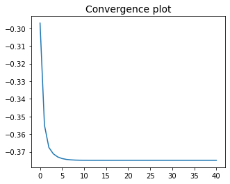
5.7.3.2.3. Numerical resolution

The optimization problem can be numerically solved with projected gradient descent in three steps

• implement the cost function with NumPy operations supported by Autograd,

• implement the projection onto the feasible set,

• select the initial point, the step-size, and the number of iterations.

All three steps are summarized in the cell below.

def cost_fun(w, tolerance=1):
    return w @ np.array(risk_matrix) @ w - tolerance * w @ np.array(expected_return)


def project_simplex(u, bound=1):
    s = np.sort(u.flat)[::-1]
    c = (np.cumsum(s) - bound) / np.arange(1, np.size(u)+1)
    l = np.max(c)
    p = np.maximum(0, u - l)
    return p


n = len(risk_matrix)
init = np.ones(n) / n
alpha = 1 / np.linalg.norm(risk_matrix, ord=2)
epochs = 40

    
w, history = gradient_descent(cost_fun, init, alpha, epochs, project_simplex)

5.7.3.2.4. Analysis

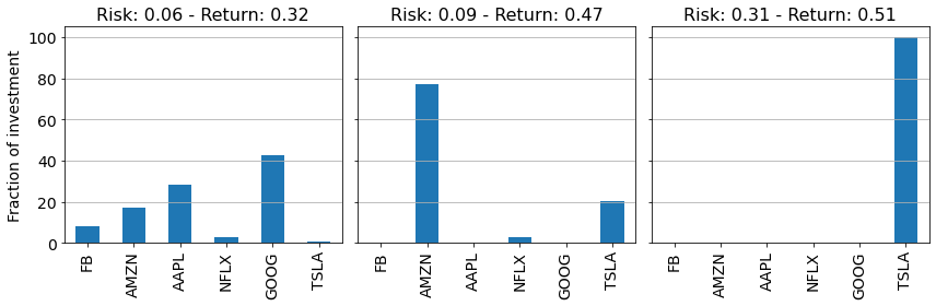
The figure below shows the optimal solution obtained with three different values for the “risk-tolerance” parameter.

• \(\gamma=0 \;\implies\) Optimal portfolio with the lowest risk.

• \(\gamma=1 \;\implies\) Optimal portfolio with medium risk.

• \(\gamma=10\!\implies\) Optimal portfolio with high risk.

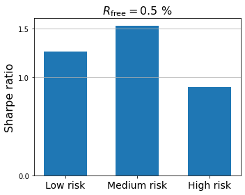
5.7.3.2.5. Sharpe ratio

In finance, the Sharpe ratio (also known as the reward-to-variability ratio) measures the performance of a portfolio compared to a risk-free asset after adjusting for its risk. It characterizes how well a portfolio’s return compensates the investor for the risk taken. Assume that \(R_{\rm free}>0\) is the return of an investment with no risk, such as a U.S. Treasury security, a “Livret A” french savings account, etc. The Sharpe ratio is then defined as the return of a portfolio minus the risk-free return and divided by the portfolio’s volatility:

\[ {\sf Sharpe}\big({\bf w}, R_{\rm free}\big) = \frac{{\bf r}^\top {\bf w} - R_{\rm free}}{\sqrt{{\bf w}^\top C {\bf w}}}. \]

The figure below compares the Sharpe ratio of the three optimal portfolios previously assembled through mean-variance optimization. The higher the Sharpe ratio, the better. As a reference, Berkshire Hathaway had a Sharpe ratio of 0.76 for the period 1976 to 2011, higher than any other stock or mutual fund with a history of more than 30 years. The stock market had a Sharpe ratio of 0.39 for the same period.

5.7.3.2.6. Known limitations

In general, there is no reason to expect that solutions to the Markowitz model will be well diversified portfolios. In fact, this model tends to produce portfolios with unreasonably large weights in certain assets. This issue is well documented in the literature, and is often attributed to estimation errors. Estimates that may be slightly off may lead the optimizer to chase phantom low-risk high return opportunities by taking large positions. Hence, portfolios chosen by “mean-variance optimization” may be subject to idiosyncratic risk. Practitioners often use additional constraints to insure themselves against estimation and model errors, as well as to ensure that the chosen portfolio is well diversified.

5.7.3.3. Conclusion

Portfolio optimization can be summarised as follows: is there a way of combining assets to produce superior risk-adjusted returns compared to a market-cap weighted benchmark? The answer is affirmative, but with some major caveats. Given the expected returns and the covariance matrix of candidate assets, one can find the portfolio that maximises the Sharpe ratio. But because we don’t know the expected returns or the future covariance matrix, we commonly replace these with the mean historical return and the sample covariance matrix. The problem is that these are very noisy estimators, so much so that a significant body of research suggests that the 1/N diversification strategy (giving each asset equal weight) outperforms most weighting schemes. Fortunately, recent studies observe that minimum-variance portfolios can beat 1/N diversification and a market-cap weighted benchmark. The nice thing about minimum-variance optimisation is that success largely depends on how well you can estimate the covariance matrix, which is easier than estimating future returns. A sensible choice is to use a shrinkage estimator of the covariance matrix, whose Python implementation can be found here.