2.4. Global optimization#
To find the minimum of a function, we as humans can simply draw the function and determine “by eye” where the smallest point lies. This visual approach can be numerically implemented by evaluating a function over a large number of its input points, and designating the input that provides the smallest value as our approximate global minimum. There are numerous ways of cleverly selecting the points over which the function is being evaluate, which distinguish gloal optimization schemes from one another. In this section, we will discuss one specific strategy called grid search.
2.4.1. Grid search#
The most trivial strategy to approximatively find the global minimum of a function is as follows.
Select a number of different points \({\bf w}_1, \dots, {\bf w}_K\).
Evaluate the function at every point, yielding a list of scalar values \(J({\bf w}_1), \dots, J({\bf w}_K)\),
Find the point \({\bf w}^\star\) that provides the lowest function value \(J({\bf w}^\star) \le J({\bf w}_k)\) for all \(k\).
This is a global optimization method called grid search. Let’s review its steps in more detail.
2.4.1.1. Step 1 - Sampling#
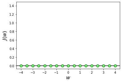
How do we choose the points \({\bf w}_1, \dots, {\bf w}_K\) on which to evaluate the cost function? We clearly cannot try them all, even for a one-dimensional function, since there are an infinite number of points to try for any continuous function. The only way is to select a finite set of points, , either by sampling them over an evenly spaced grid, or by picking them at random. This approach is illustrated in the next figure, where the green dots mark the points sampled from the interval \([-4,4]\).
2.4.1.2. Step 2 - Evaluation#
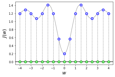
Once the candidates \({\bf w}_1, \dots, {\bf w}_K\) are selected, we can proceed to evaluate the cost function \(J({\bf w})\) on each of them, so as obtain a list of values \(J({\bf w}_1), \dots, J({\bf w}_K)\). This is illustrated in the next figure, where the blue dots mark the values of the cost function evaluated at the points selected in the previous step.
2.4.1.3. Step 3 - Optimization#
When the evalutions \(J({\bf w}_1), \dots, J({\bf w}_K)\) are obtained for every candidate, we can determine the point that (approximatively) optimizes the function \(J({\bf w})\). This step boils down to computing the minimum over a finite set of values:
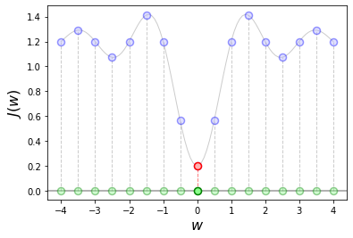
In short, we select the point \({\bf w}_{k^*}\) corresponding to the smallest cost among \(J({\bf w}_1), \dots, J({\bf w}_K)\). This is the red point highlighted in the figure below, which in this example appears to lie very close to the actual minimum of the function.
2.4.2. Numerical implementation#
The following is a Python implementation of grid search. Notice that each step of the algorithm is translated into one or several lines of code. Numpy library is used to vectorize operations whenever possible.
def grid_search(cost_fun, wmin, wmax, n_points):
    """
    Finds the minimum of a function.

    Arguments:
    cost_fun -- cost function    | callable that takes 'w' and returns 'J(w)'
    wmin     -- min values       | vector of shape (N,)
    wmax     -- max values       | vector of shape (N,)
    n_points -- number of points | integer

    Returns:
    w -- minimum point | vector of shape (N,)
    """
    wmin = np.array(wmin)
    wmax = np.array(wmax)

    # Step 1. Generate some random points between 'wmin' and 'wmax'
    points = np.random.rand(n_points, wmin.size) * (wmax - wmin) + wmin

    # Step 2. Evaluate the function on the generated points
    costs = [cost_fun(w) for w in points]

    # Step 3. Select the point with the lowest cost
    k = np.argmin(costs)
    w = points[k]

    return w
The python implementation requires three arguments:
the function to optimize,
a rough interval that limits the search space of each variable,
the number of points to be searched.
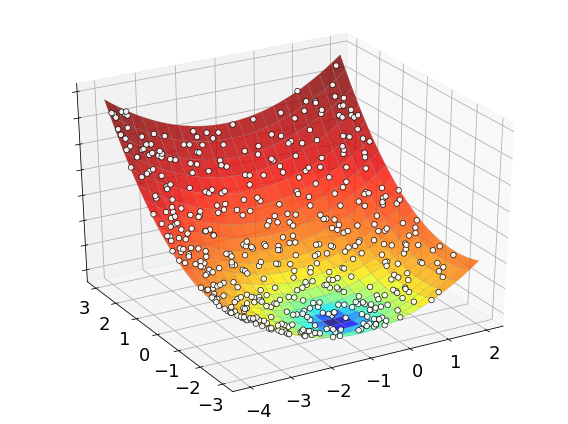
The result is the point where the function attains its smallest value among all the randomly selected candidates. An usage example is presented next.
# cost function of two variables
cost_fun = lambda w: (w[0]+1)**2 + (w[1]+2)**2

# rough intervals of the search space
wmin = [-4, -3]
wmax = [ 2,  3]

# number of points to explore
n_points = 500

# numerical optimization
w, points = grid_search(cost_fun, wmin, wmax, n_points)
The process of optimizing a function with grid search is illustrated below. The white dots mark all the candidates evaluated by the algorithm to find its final approximation of the minimum point.
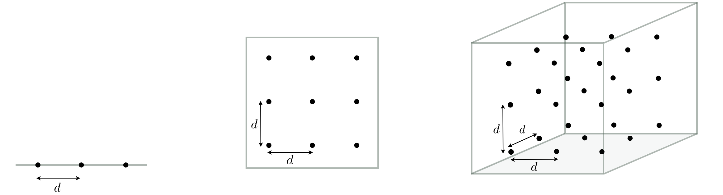
2.4.3. Curse of dimensionality#
Global optimization by grid search is easy to implement and perfectly adequate for low-dimensional functions. However, it fails miserably as we try to tackle functions of larger dimensions. To get a sense of why this approach quickly becomes infeasible, let’s consider the following scenario. Imagine that we have a one-dimensional function, and we sample 3 points that are precisely at a distance \(d\) from one another (this is illustrated in the left panel of the figure below). Imagine now that the function dimension increases by one, and that we increase the samples so as to keep a distance of \(d\) between closest neighbors (as illustrated in the middle panel below). However, in order to do this in two-dimensional space, we need to sample \(3^2=9\) points. Likewise, if we increase the function dimension once again in the same fashion to sample evenly across the solution space so as to keep the same distance \(d\) between closest neighbors, we will need \(3^3=27\) points (as illustrated in the right panel below). More generally, if we continue this for a general N-dimensional space, we would need to sample \(3^N\) points, a huge number even for moderate sized N. This is an example of the so-called curse of dimensionality, which describes the exponential difficulty we encounter when trying to deal with functions of increasing dimension. The issue here is that we want to keep the distance \(d\) small in order to precisely locate the optimum point \(w^*\), which however requires us to sample exponentially many points to keep up with the increase of dimensionality.