5.4. Orthogonal projection

An interesting problem is to find the point of a subset that is located at the smallest possible distance from a given point. The solution to this particular type of constrained optimization problem is called orthogonal projection. It generalizes the notion of projection from linear algebra, and it is a building block of many constrained optimization algorithms.

1 - Definition. The orthogonal projection of a point \({\bf u}\in\mathbb{R}^N\) onto a subset \(\mathcal{C}\subset \mathbb{R}^N\) is formally defined as

\[ \mathcal{P}_{\mathcal{C}}({\bf u}) \in \operatorname*{Argmin}_{{\bf w}\in\mathcal{C}}\; \|{\bf w}-{\bf u}\|^2. \]

In general, there may exist several orthogonal projections of a point onto a set, provided that the latter is nonempty and closed. The above \(\operatorname{Argmin}\) (with uppercase ‘A’) denotes the set of all the points of \(\mathcal{C}\) at the same smallest distance from \({\bf u}\), and the inclusion symbol (\(\in\)) is there to remind that the orthogonal projection \(\mathcal{P}_{\mathcal{C}}({\bf u})\) can be any of those points.

2 - Convexity. The orthogonal projection is unique when the set \(\mathcal{C}\) is convex. In this case, the projection can be precisely defined as the unique point of \(\mathcal{C}\) at the smallest distance from \({\bf u}\) (note the \(\operatorname{argmin}\) is now with lowercase ‘a’):

\[ \textrm{$\mathcal{C}\,$ is convex} \qquad\implies\qquad \mathcal{P}_{\mathcal{C}}({\bf u}) = \operatorname*{argmin}_{{\bf w}\in\mathcal{C}}\; \|{\bf w}-{\bf u}\|^2 \;\; \textrm{is unique}. \]

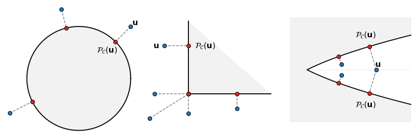
3 - Geometrical optimality. In any case, the necessary optimality condition states that the direction from the projection \(\mathcal{P}_{\mathcal{C}}({\bf u})\) to the original point \({\bf u}\) is orthogonal to the set \(\mathcal{C}\) at \(\mathcal{P}_{\mathcal{C}}({\bf u})\):

\[ {\bf u} - \mathcal{P}_{\mathcal{C}}({\bf u}) \in \mathcal{N}_{\mathcal{C}}\big(\mathcal{P}_{\mathcal{C}}({\bf u})\big). \]

This explains why it is called “orthogonal projection”. Some examples are illustrated below.

4 - Properties. Open the sections below to learn more about the orthogonal projection and its various properties.

Idempotence

By looking at the definition, it is immediately evident that any point of \(\mathcal{C}\) is the projection of itself:

\[ {\bf w} \in \mathcal{C} \qquad\Longrightarrow\qquad \mathcal{P}_{\mathcal{C}}({\bf w}) = {\bf w}. \]

The projection is thus an idempotent operation, because \(\mathcal{P}_{\mathcal{C}}(\mathcal{P}_{\mathcal{C}}({\bf u})) = \mathcal{P}_{\mathcal{C}}({\bf u})\) for any point \({\bf u} \in \mathbb{R}^N\).

Cartesian product

A constraint of \(\mathbb{R}^{N}\) may be defined as the cartesian product of several sets \(\mathcal{C}_k\subset \mathbb{R}^{N_k}\) of smaller dimensions such that \(N=N_1+\dots+N_K\), namely

\[ \mathcal{C}_{\rm prod} = \mathcal{C}_1 \times \mathcal{C}_2 \times \dots\times \mathcal{C}_K. \]

A vector of \(\mathcal{C}_{\rm prod}\) is decomposed in blocks, and each block belongs to the corresponding \(\mathcal{C}_k\):

\[\begin{split} {\bf w} = \begin{bmatrix} {\bf w}_1 \\ \vdots \\ {\bf w}_K \end{bmatrix} \in \mathcal{C}_{\rm prod} \qquad\Longleftrightarrow\qquad \begin{cases} {\bf w}_1 \in \mathcal{C}_1 \\ \quad\;\vdots \\ {\bf w}_K \in \mathcal{C}_K. \\ \end{cases} \end{split}\]

Then, the projection onto \(\mathcal{C}_{\rm prod}\) concatenates the projections onto each \(\mathcal{C}_k\):

\[\begin{split} \mathcal{P}_{\mathcal{C}_{\rm prod}}({\bf u}) = \begin{bmatrix} \mathcal{P}_{\mathcal{C}_1}({\bf u}_1)\\ \vdots\\ \mathcal{P}_{\mathcal{C}_K}({\bf u}_K)\\ \end{bmatrix}. \end{split}\]

Intersection

A constraint of \(\mathbb{R}^{N}\) may be defined as the intersection of several sets \(\mathcal{C}_k\subset \mathbb{R}^{N}\) of equal dimension:

\[ \mathcal{C}_{\rm cross} = \mathcal{C}_1 \cap \mathcal{C}_2 \cap \dots\cap \mathcal{C}_K. \]

A vector of \(\mathcal{C}_{\rm cross}\) belongs to all \(\mathcal{C}_k\) simultaneously:

\[\begin{split} {\bf w} \in \mathcal{C}_{\rm cross} \qquad\Longleftrightarrow\qquad \begin{cases} {\bf w} \in \mathcal{C}_1 \\ \quad\!\vdots \\ {\bf w} \in \mathcal{C}_K. \\ \end{cases} \end{split}\]

The projection onto \(\mathcal{C}_{\rm cross}\) cannot be written as a simple combination of projections onto each \(\mathcal{C}_k\):

\[ \mathcal{P}_{\mathcal{C}_{\rm cross}}({\bf u}) \stackrel{\stackrel{\bf NOT\,EQUAL}{\downarrow}}{\neq} \mathcal{P}_{\mathcal{C}_1}\Big( \mathcal{P}_{\mathcal{C}_2}\big(\dots \mathcal{P}_{\mathcal{C}_K}({\bf u})\big)\Big). \]

Shift

A constraint of \(\mathbb{R}^{N}\) may be defined as the points of a set \(\mathcal{C}\subset \mathbb{R}^{N}\) shifted by a vector \({\bf r}\in\mathbb{R}^{N}\):

\[ \mathcal{C}_{\rm shift} = \begin{Bmatrix} {\bf w} \in \mathbb{R}^{N} \;|\; {\bf w} - {\bf r}\in \mathcal{C} \end{Bmatrix}. \]

The projection onto \(\mathcal{C}_{\rm shift}\) is related to the projection onto \(\mathcal{C}\) by a simple shift:

\[ \mathcal{P}_{\mathcal{C}_{\rm shift}}({\bf u}) = {\bf r} + \mathcal{P}_{\mathcal{C}}({\bf u}-{\bf r}). \]

Linear transform

A constraint of \(\mathbb{R}^{N}\) may be defined as the points of a set \(\mathcal{C}\subset \mathbb{R}^{K}\) after a multiplication by \(A\in\mathbb{R}^{K\times N}\):

\[ \mathcal{C}_{\rm linear} = \begin{Bmatrix} {\bf w} \in \mathbb{R}^{N} \;|\; A {\bf w} \in \mathcal{C} \end{Bmatrix}. \]

If \(A\) is a \(\nu\)-frame with \(\nu>0\), the projection onto \(\mathcal{C}_{\rm linear}\) is related to the projection onto \(\mathcal{C}\) as follows:

\[ A A^\top=\nu I_{K\times K} \quad\Rightarrow\quad \mathcal{P}_{\mathcal{C}_{\rm linear}}({\bf u}) = %{\bf r} + \mathcal{P}_{\mathcal{C}}({\bf u}-{\bf r}). {\bf u} + \frac{1}{\nu} A^\top\big( \mathcal{P}_{\mathcal{C}}(A{\bf u}) - A{\bf u} \big). \]

Note that NO formula exists in the general case when \(A A^\top \neq \nu I\).

Spectral sets

When the optimization is taken with respect to symmetric (square) matrices, a constraint of \(\mathbb{R}^{N\times N}\) may be defined as the matrices with eigenvalues belonging to a set \(\mathcal{C}\subset \mathbb{R}^{N}\):

\[ \mathcal{C}_{\rm eig} = \begin{Bmatrix} W \in \mathbb{R}^{N\times N} \;|\; \lambda_W \in \mathcal{C} \end{Bmatrix}, \]

where \(\lambda_W\in\mathbb{R}^{N}\) denotes the vector of eigenvalues of \(W\). The projection onto \(\mathcal{C}_{\rm eig}\) is related to the projection onto \(\mathcal{C}\) as follows:

\[ \mathcal{P}_{\mathcal{C}_{\rm eig}}(U) = Q_U\,{\rm diag}\big(\mathcal{P}_{\mathcal{C}}(\lambda_U)\big)\,Q_U^\top. \]

where \(U=Q_U\,{\rm diag}(\lambda_U)\,Q_U^\top\) is a spectral decomposition of \(U\). When the optimization is taken with respect to rectangular matrices, the singular value decomposition replaces the spectral decomposition.