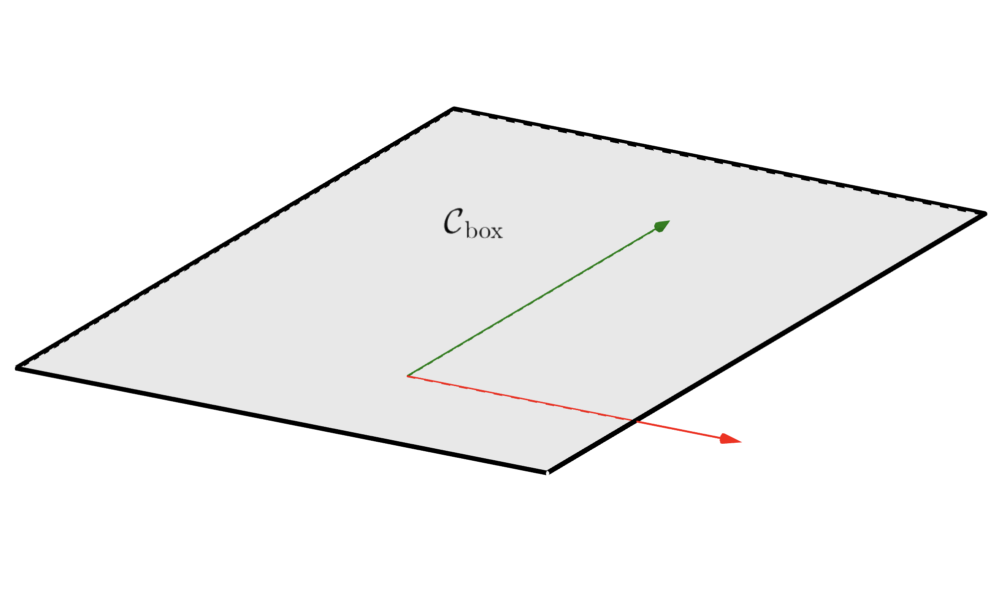
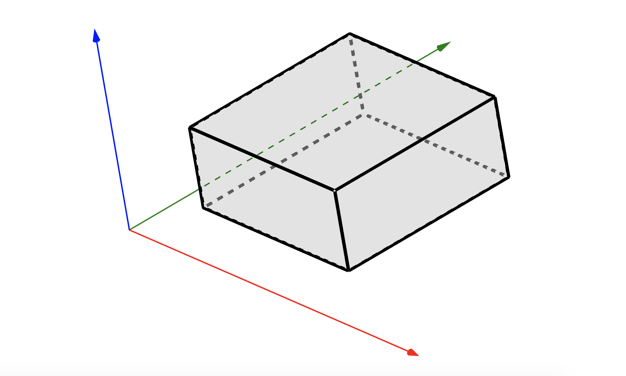
5.4.1. Box

Given the scalars \(a_i \in \mathbb{R} \cup \{-\infty\}\) and \(b_i \in \mathbb{R} \cup \{+\infty\}\), the box is a linear constraint defined as

\[ \mathcal{C}_{\rm box} = \big\{ {\bf w} \in \mathbb{R}^{N} \;|\; a_i \le w_i \le b_i \quad (i = 1,\dots,N) \big\}. \]

The condition \(a_i \le b_i\) is required for this subset to be nonempty, possibbly with \(a_i=-\infty\) or \(b_i=+\infty\) to drop some of the lower/upper bounds. The figure below shows how this constraint looks like in \(\mathbb{R}^{2}\) or in \(\mathbb{R}^{3}\).

Box in 2D

Box in 3D

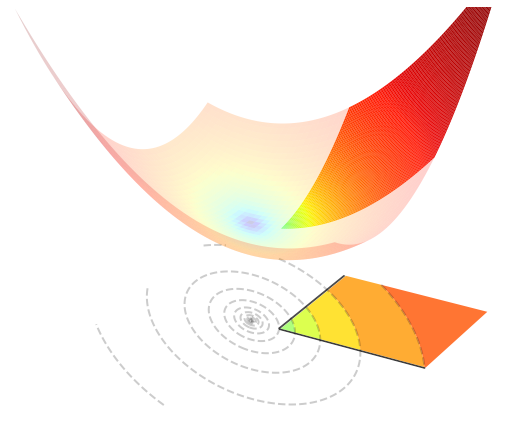
5.4.1.1. Constrained optimization

Optimizing a function \(J({\bf w})\) subject to the box constraint can be expressed as

\[ \operatorname*{minimize}_{\textbf{w}\in\mathbb{R}^N}\;\; J({\bf w}) \quad{\rm s.t.}\quad a_i \le w_i \le b_i \quad (i = 1,\dots,N). \]

Defining the vectors \({\bf a} = [a_1, \dots, a_N]^\top\) and \({\bf b} = [b_1, \dots, b_N]^\top\) allows one to render the box constraint as a single liner \({\bf a} \le {\bf w} \le {\bf b}\), so that the above problem can be compactly written as

\[ \operatorname*{minimize}_{\textbf{w}\in\mathbb{R}^N}\;\; J({\bf w}) \quad{\rm s.t.}\quad {\bf a} \le {\bf w} \le {\bf b}. \]

The figure below visualizes such an optimization problem in \(\mathbb{R}^{2}\).

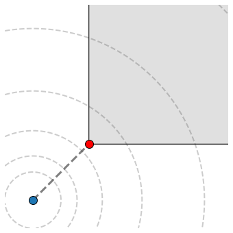
5.4.1.2. Orthogonal projection

The projection of a point \({\bf u}\in\mathbb{R}^{N}\) onto the box is the (unique) solution to the problem

\[\begin{split} \operatorname*{minimize}_{{\bf w}\in\mathbb{R}^N}\;\; \|{\bf w}-{\bf u}\|^2 \quad{\rm s.t.}\quad {\bf a} \le {\bf w} \le {\bf b}. %a_i \le w_i \le b_i \quad (i=1,\dots,N) %\begin{cases} %a_1 \le w_1 \le b_1\\ %\qquad\;\vdots\\ %a_N \le w_N \le b_N. %\end{cases} \end{split}\]

The solution can be analytically computed as follows.

Projection onto the box

\[\begin{split} \mathcal{P}_{\mathcal{C}_{\rm box}}({\bf u}) = \max\{{\bf a}, \min\{{\bf u}, {\bf b}\}\} = \begin{bmatrix} \max\{a_1, \min\{u_1, b_1\}\}\\ \vdots\\ \max\{a_N, \min\{u_N, b_N\}\}\\ \end{bmatrix} \end{split}\]

The next figure visualizes a point \({\bf u}\in \mathbb{R}^{2}\) (blue dot) along with its projection (red dot) onto this set.

5.4.1.3. Implementation

The python implementation is given below.

def project_box(u, lower=None, upper=None):
    
    assert lower is None or upper is None or np.all(lower <= upper), "Required: lower <= upper"
    
    p = np.clip(u, lower, upper)
    
    return p

Here are some examples of use.

u = np.array([-0.5, -0.5])

p1 = project_box(u, lower=0)
p2 = project_box(u, upper=0)
p3 = project_box(u, lower=[0,-np.Inf], upper=[np.Inf, 1])