5.3. Geometric optimality

Constrained optimization aims at finding a minimum of the function \(J({\bf w})\) on the feasible set \(\mathcal{C}\subset \mathbb{R}^N\), formally denoted as

\[ \operatorname*{minimize}_{{\bf w}\in\mathbb{R}^N}\quad J({\bf w}) \quad\textrm{subject to}\quad {\bf w}\in\mathcal{C}. \]

The solutions to a constrained optimization problem can be precisely characterized by putting the gradient of \(J({\bf w})\) in relation to the topology of \(\mathcal{C}\), yielding what are called the first-order constrained optimality conditions.

5.3.1. Constrained minimum

A point \({\bf w}^\star\!\in\mathcal{C}\) that gives the smallest value of \(J({\bf w})\) on the set \(\mathcal{C}\) is called constrained “global” minimum.

Constrained “global” minimum

\[ {\bf w}^\star\in\mathcal{C} \quad\textrm{such that}\quad (\forall{\bf w}\in\mathcal{C})\quad J({\bf w}^\star) \le J({\bf w}) \]

Constrained “local” minimum

The goal of constrainted optimization is to retrieve a solution that is globally optimal. This may not always be possible, depending on the “difficulty” of a given problem. In such cases, we are forced to settle for a solution that is only locally optimal. In this regard, a constrained “local” minimum is a point \({\bf \bar{w}}\in\mathcal{C}\) that gives the smallest value of \(J({\bf w})\) on the intersection of \(\mathcal{C}\) with a sufficiently small neighbor \(\mathcal{B}_r\) of \({\bf \bar{w}}\), namely

\[ \textrm{${\bf \bar{w}}$ is a local minimum of $J({\bf w})$ on $\mathcal{C}$}\qquad\Leftrightarrow\qquad %{\bf \bar{w}}\in\mathcal{C} %\quad{\rm and}\quad \big(\exists r > 0 : \forall{\bf w}\in\mathcal{C}\cap\mathcal{B}_r({\bf \bar{w}})\big)\quad J({\bf \bar{w}}) \le J({\bf w}). \]

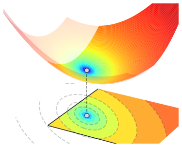
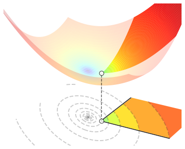
By definition, a constrained minimum occurs

• either at a proper minimum of the function \(J({\bf w})\) - if such minimum belongs to \(\mathcal{C}\),

• or at the boundary of the feasible set \(\mathcal{C}\) - if none of the function’s proper minima belong to \(\mathcal{C}\).

Both of these situations are illustrated in the figure below. In the left panel, the proper minimum of \(J({\bf w})\) belongs to \(\mathcal{C}\), and thus it is also the constrained minimum of \(J({\bf w})\) on \(\mathcal{C}\). In the right panel, the proper minimum of \(J({\bf w})\) does not belong to \(\mathcal{C}\), hence it cannot be the constrained minimum of \(J({\bf w})\) on \(\mathcal{C}\). The latter is instead located somewhere at the boundary of \(\mathcal{C}\).

Solution at the interior of the feasible set

Solution at the boundary of the feasible set

A solution to a constrained optimization problem may not always exist. The foremost assumption in constrained optimization is that the feasible set \(\mathcal{C}\) must be nonempty and closed, so as to ensure that \(\mathcal{C}\) contains its boundary. Hovewer, this is usually not enough to guarantee the existence of a constrained minimum, and some additional hypotheses are required on both the function \(J({\bf w})\) and the feasible set \(\mathcal{C}\), such as the following ones. [1]

Existence of constrained minima

\[\begin{split} \begin{cases} \textrm{$\mathcal{C}\subset \mathbb{R}^N$ is nonempty and closed}\\ \textrm{$J({\bf w})$ is continuous on $\mathcal{C}$}\\ \textrm{$J({\bf w})$ is coercive}\;{\bf or}\; \textrm{$\mathcal{C}$ is bounded}\\ \end{cases} \qquad\implies\quad \textrm{There exists a minimum of $J({\bf w})$ on $\mathcal{C}$}. \end{split}\]

This is a sufficient condition. A constrained minimum may exist even if the above assumptions do not hold.

5.3.2. Geometric insights

Constrained optimization is based on the following intuition. If the point \({\bf w}^\star\in\mathcal{C}\) is a minimum of \(J({\bf w})\) on \(\mathcal{C}\), then it should not be possible to decrease the function along any path inside \(\mathcal{C}\) starting at \({\bf w}^\star\). Since the function can be locally decreased by moving in any direction whose angle is less than \(90°\) with respect to the negative gradient \(-\nabla J({\bf w})\), optimality occurs only in two different cases:

• either the gradient \(\nabla J({\bf w}^\star)\) is zero,

• or the negative gradient \(-\nabla J({\bf w}^\star)\) is orthogonal to \(\mathcal{C}\) at \({\bf w}^\star\).

Such concept is illustrated in the following examples.

Note

A function decreases locally in any direction whose angle is less than \(90°\) to the negative gradient.

5.3.2.1. Constraint with “smooth” boundary

The figure below presents the constrained optimization problem

\[ \operatorname*{minimize}_{{\bf w}\in\mathbb{R}^2}\; \|A{\bf w} - {\bf b}\|^2\quad{\rm s.t.}\quad \|{\bf w}\|_2\le 1. \]

Since the function’s smallest point falls outside the constraint, the constrained minimum lies on the boundary (white dot). By moving the slider from left to right, you can visualize the negative gradient (black/red arrow) on differents points of the boundary (red dot). The constrained minimum is the point where the negative gradient forms a 90° angle with the line tangent to the constraint at that point (green line). This condition ensures that the function cannot be further decreased by moving to any other point that satisfies the constraint.

Note

The gradient \(\nabla J({\bf w})\) is always orthogonal to the contour lines of \(J({\bf w})\).

Once Loop Reflect

5.3.2.2. Constraint with “corners”

The boundary of a constraint may not be smooth everywhere. For example, consider the constrained optimization problem

\[ \operatorname*{minimize}_{{\bf w}\in\mathbb{R}^2}\; \|A{\bf w} - {\bf b}\|^2\quad{\rm s.t.}\quad {\bf w} \ge 0. \]

As you can see in the figure below, the non-negative constraint features a “corner” at the point \((0,0)\), which is also the constrained minimum of the problem (white dot). To check for optimality in this case, one must consider the two side directions (green arrows) that are tangent to the boundary at a given point (red dot), and look at the angles they form with the negative gradient (black/red arrow). By moving the slider to the right, you can see that 119° and 151° are the angles formed at \((0,0)\). This happens because the two side directions wrap around the corner at \((0,0)\) to remain tangential to the boundary. Since both angles are \(\ge 90°\), all the descent directions (gray cone) are oriented outward the constraint, and the function cannot be further decreased by moving along the boundary or inward the constraint.

Once Loop Reflect

5.3.3. First-order conditions

The geometric intuition behind constrained optimization can be mathematically formalized through the normal cone. The latter indeed describes the geometrical situation where “a vector is orthogonal to a set (at a given point)”, namely

\[\begin{split} {\bf d}\in \mathcal{N}_{\mathcal{C}}({\bf w}) \quad\Leftrightarrow\quad \begin{cases} {\bf d}={\bf 0}\\ \;\;\;{\rm or}\\ \textrm{${\bf d}$ is orthogonal to $\mathcal{C}$ at ${\bf w}$.} %\small \textrm{${\bf d}$ forms an angle $\ge 90°$ with every tangential direction of $\mathcal{C}$ at ${\bf w}$}. \end{cases} \end{split}\]

The following conditions will simply use the normal cone to restate the fact that optimality arises when the negative gradient is either zero or orthogonal to the constraint.

5.3.3.1. Necessary optimality condition

The necessary optimality condition states that if the point \({\bf w}^\star\) is a minimum of \(J({\bf w})\) on \(\mathcal{C}\), then the negative gradient \(-\nabla J({\bf w}^\star)\) must belong to the normal cone of \(\mathcal{C}\) at \({\bf w}^\star\).

First-order optimality (necessary)

\[ \textrm{${\bf w}^\star$ is a minimum of $J({\bf w})$ on $\mathcal{C}$} \quad\implies\quad -\nabla J({\bf w}^\star) \in \mathcal{N}_{\mathcal{C}}({\bf w}^\star). \]

The above necessary condition is twofold.

• When a constrained minimum occurs on the boundary of \(\mathcal{C}\), the negative gradient is orthogonal to \(\mathcal{C}\) there.

• When a constrained minimum occurs in the interior of \(\mathcal{C}\), the gradient is zero there, because the normal cone only contains the zero vector, and the above inclusion reverts to the well-known equality \(\nabla J({\bf w}^\star)={\bf 0}\).

Note that being a necessary condition, there may exist points \(\bar{{\bf w}}\) satisfying the inclusion \(-\nabla J(\bar{{\bf w}}) \in \mathcal{N}_{\mathcal{C}}(\bar{{\bf w}})\) that are not global minima. Nonconvex constraints often lead to the presence of such points, even if the objective function is convex.

Constrained “stationary” point

In relation to nonconvex constrained problems, one may wonder what are all those points \(\bar{{\bf w}}\) such that \(-\nabla J(\bar{{\bf w}}) \in \mathcal{N}_{\mathcal{C}}(\bar{{\bf w}})\). They are all the global and local constrained minima, maxima, and saddles of \(J({\bf w})\) on \(\mathcal{C}\), as shown in the example below. These are collectively called constrained “stationary” points, because there exists no feasible descent direction at any of these points.

\[ -\nabla J(\bar{{\bf w}}) \in \mathcal{N}_{\mathcal{C}}(\bar{{\bf w}}) \quad\iff\quad \textrm{${\bf \bar{w}}$ is a stationary point of $J({\bf w})$ on $\mathcal{C}$}. \]

The figure below shows an optimization problem with a nonconvex equality constraint. By moving the slider from left to right, you can visualize the negative gradient (black/red arrow) and the normal cone (pink area) on differents points of the boundary (red dot). Since the white point is the constrained global minimum, the negative gradient aligns with the normal cone there, which is equivalent to say that the negative gradient is “orthogonal” to the constraint. However, the orthogonality triggers in three other points, namely a constrained local minimum (gray square), and two constrained maxima (yellow stars). This is why the aforementioned optimality condition is merely “necessary” and not “sufficient”.

Here is a 3D representation of the optimization problem, where the constrained minima/maxima can be clearly seen.

5.3.3.2. Sufficient optimality condition

Constrained optimization is greatly simplified when both \(J({\bf w})\) and \(\mathcal{C}\) are convex. Why do we care about convexity? Because it ensures that every point in which the negative gradient is “orthogonal” to the constraint results in a constrained global minimum. This fact can be summarized as follows.

First-order optimality (sufficient)

\[\begin{split} \begin{cases} -\nabla J({\bf w}^\star) \in \mathcal{N}_{\mathcal{C}}({\bf w}^\star)\\[0.5em] \textrm{$J({\bf w})$ and $\mathcal{C}$ are convex} \end{cases} \quad\Rightarrow\quad \textrm{${\bf w}^\star$ is a minimum of $J({\bf w})$ on $\mathcal{C}$}. \end{split}\]

The figure below illustrates the sufficient optimality condition on a convex constrained problem. By moving the slider from left to right, you can visualize the negative gradient (black/red arrow) and the normal cone (pink area) on differents points of the boundary (red dot). The constrained minimum is the point where the negative gradient overlaps with the normal cone, which happens precisely at the corner point (white dot). This is equivalent to say that the negative gradient is “orthogonal” to the constraint at the solution.

Once Loop Reflect

5.3.4. Appendix

The descent directions of a function \(J({\bf w})\) at a point \({\bf w}\) are all the vectors whose angle is less than \(90°\) with respect to the negative gradient at \({\bf w}\), namely

\[ \mathcal{D}_{J}({\bf w}) = \big\{{\bf p}\in \mathbb{R}^N \;|\; \underbrace{-\nabla J({\bf w})^\top{\bf p}>0}_{\scriptsize{\rm angle}(-\nabla J({\bf w}),\,{\bf p})\,<\,90°}\big\}. \]

Intuitively, if \({\bf w}^\star\) is a minimum of \(J({\bf w})\) on \(\mathcal{C}\), then the cone of descent directions does not intersect with the tangent cone:

\[ \textrm{${\bf w}^\star$ is a minimum of $J({\bf w})$ on $\mathcal{C}$} \quad\Rightarrow\quad \mathcal{D}_{J}({\bf w}^\star) \cap \mathcal{T}_{\mathcal{C}}({\bf w}^\star) = \emptyset. \]

The empty intersection means that all the descent directions at \({\bf w}^\star\) are oriented to the outside of \(\mathcal{C}\), because there exists no feasible direction at \({\bf w}^\star\) to reduce the function value \(J({\bf w}^\star)\).

An equivalent condition is to say that the negative gradient \(-\nabla J({\bf w}^\star)\) forms an angle \(\ge 90°\) with all the vectors in the tangent cone at \({\bf w}^\star\). This fact can be exactly expressed through an inclusion into the normal cone. Therefore, the relationship between normal, tangent, and descent cones can be summarized by the following equivalence:

\[ \mathcal{D}_{J}({\bf w}) \cap \mathcal{T}_{\mathcal{C}}({\bf w}) = \emptyset \quad\Leftrightarrow\quad -\nabla J({\bf w}) \in \mathcal{N}_{\mathcal{C}}({\bf w}). \]

The necessary optimality condition can be thus recovered by putting together the two statements:

\[ \textrm{${\bf w}^\star$ is a minimum of $J({\bf w})$ on $\mathcal{C}$} \quad\Rightarrow\quad -\nabla J({\bf w}) \in \mathcal{N}_{\mathcal{C}}({\bf w}). \]

---

[1]

The result still holds if continuity is replaced by lower semi-continuity.