2.2. Objective function

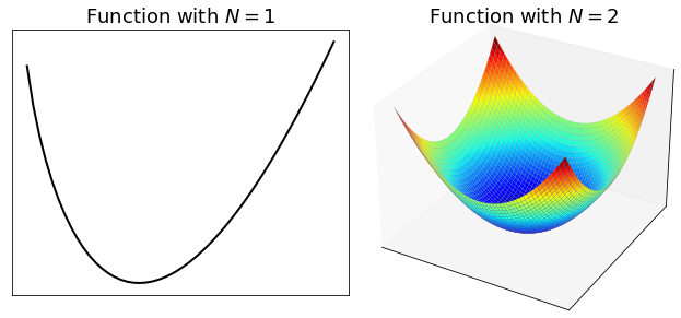
The function to be minimized or maximized in an optimization problem is called objective function, cost function (only for minimization), or utility function (only for maximization). It is a function from \(\mathbb{R}^N\) to \(\mathbb{R}\) that takes as input \(N\) real numbers, and produces a real number as output. Throughout the course, the objective function will be conventionally denoted as

\[ J\colon\mathbb{R}^N\to\mathbb{R}. \]

The domain \(\mathbb{R}^N\) indicates that the function’s “input” is a vector of real variables denoted as

\[\begin{split} {\bf w} = \begin{bmatrix} w_1\\ w_2\\ \vdots\\ w_N \end{bmatrix} \in \mathbb{R}^N, \end{split}\]

and the codomain \(\mathbb{R}\) indicates that the function’s “output” is a real number denoted as \(J(\bf w)\) or equivalently \(J(w_1, w_2, \dots,w_N)\). The figure below shows two examples of function.

2.2.1. Continuity

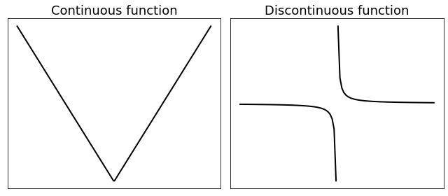
A function is continuous if it does not have any abrupt changes in value. More precisely, a function \(J({\bf w})\) is continuous at some point \(\bar{\bf w}\) of its domain, if the limit of \(J({\bf w})\), as \({\bf w}\) approaches \(\bar{\bf w}\) through the domain of \(J\), exists and is equal to \(J(\bar{\bf w})\).

Continuity

\[ \lim_{{\bf w}\to\bar{\bf w}} J({\bf w}) = J(\bar{\bf w}). \]

The function (as a whole) is said to be continuous, if it is continuous at every point of its domain. Roughly speaking, a continuous function can be drawn as a single unbroken curve (or surface) over all its domain. A function is said to be discontinuous at some point when it is not continuous there. The figure below shows examples of continuous and discontinuous functions.

2.2.2. Coercivity

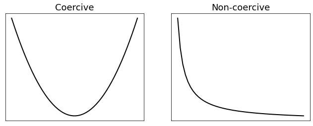
A function is coercive if it grows to infinity at the extremes of the space on which it is defined.

Coercivity

\[ \lim_{\|{\bf w}\|\to+\infty} J({\bf w}) = +\infty \]

The figure below shows an example of coercive function (left side) and non-coercive function (right side).

2.2.3. Convexity

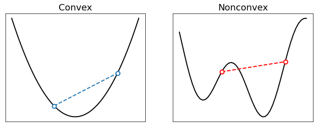
A function is convex if its graph “curves up” without any bend the other way. More precisely, a convex function meets the following inequality

\[ \big(\forall{\bf x},{\bf y}\in{\rm dom}(J), \forall t \in [0,1]\big) \qquad J\big(t {\bf x} + (1-t) {\bf y}\big) \le t J({\bf x}) + (1-t) J({\bf y}). % %\big(\forall{\bf x},{\bf y}\in{\rm dom}(f)\big) \qquad f\left(\frac{{\bf x} + {\bf y}}{2}\right) \le \frac{f({\bf x}) + f({\bf y})}{2}. \]

The above definition has a simple geometric interpretation: the segment connecting \(({\bf x}, J({\bf x}))\) to \(({\bf y}, J({\bf y}))\) never goes under the graph of \(J\). See the examples below.

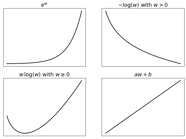
Here are several examples of convex functions.

• \(f(w) = e^{w}\)

• \(f(w) = |x|^{a}\) with \(a\ge 1\)

• \(f(w) = x^{-a}\) over \(\mathbb{R}_{++}\) with \(a\ge0\)

• \(f(w) = -\sqrt[a]{x}\) over \(\mathbb{R}_{++}\) with \(a>0\)

• \(f(w) = -\log w\) over \(\mathbb{R}_{++}\)

• \(f(w) = x\log x\) over \(\mathbb{R}_{+}\) (and \(0\log0=0\) by convention)

• \(f({\bf w}) = {\bf c}^\top {\bf w}\)

• \(f({\bf w}) = \|A {\bf w} - {\bf b}\|^2\)

• \(f({\bf w}) = {\bf w}^\top Q {\bf w}\) provided that \(Q\) is positive semi-definite

• \(f({\bf w}) = \|{\bf w}\|_p\) with \(p\ge1\)

• \(f({\bf w}) = \max\{w_1,\dots,w_N\}\)

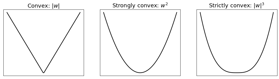
2.2.3.1. Strict convexity

A convex function is strictly convex if it has greater curvature than a linear function. Such requirement is equivalent to enforce convexity with a strict inequality

\[ \big(\forall{\bf x}\neq{\bf y}\in{\rm dom}(J), \forall t \in ]0,1[\big) \qquad J\big(t {\bf x} + (1-t) {\bf y}\big) < t J({\bf x}) + (1-t) J({\bf y}). % %\big(\forall{\bf x}\neq{\bf y}\in{\rm dom}(f)\big) \qquad f\left(\frac{{\bf x} + {\bf y}}{2}\right) < \frac{f({\bf x}) + f({\bf y})}{2}. \]

Intuitively, the above test fails when a convex function is linear somewhere on its domain. This also includes flat zones, which can only occur at the minimum of convex functions by definition.

2.2.3.2. Strong convexity

A convex function is strongly convex if it has at least the same curvature as a quadratic function. This requires the existence of a positive value \(\mu>0\) such that \(J({\bf w}) - \frac{\mu}{2}\|{\bf w}\|^2\) is still convex. Put another way, adding a quadratic term to a convex function makes it strongly convex.

\[ \textrm{$J({\bf w})$ is convex}\qquad\Rightarrow\qquad \textrm{$J({\bf w})+\frac{\mu}{2}\|w\|^2$ is strongly convex} \]

Interestingly, the three types of convexity are related.

Note

• Strong convexity \(\Rightarrow\) Strict convexity \(\Rightarrow\) Convexity

• Strong convexity \(\Rightarrow\) Coercivity

2.2.3.3. Convexity-preserving rules

To quickly recognize a convex function, it is often easier to verify that a matehatical expression contains only “convexity preserving” operations. Here is a quick overview of such operations.

• \(g({\bf x}) = w_1 f_1({\bf x}) + \dots + w_n f_n({\bf x})\) is convex if so are \(f_1,\dots, f_n\) and \(w_1, \dots, w_n \ge 0\).

\[g({\bf x}) = \sum_{i} x_i\]

• \(g({\bf x}) = \max\{f_1({\bf x}), \dots, f_n({\bf x})\}\) is convex if so are \(f_1,\dots, f_n\).

\[g({\bf x}) = \max_{i} x_i\]

• \(g({\bf x}) = f(A{\bf x}+{\bf b})\) is convex if so is \(f\), with \(A\in\mathbb{R}^{M\times N}\) and \({\bf b}\in\mathbb{R}^{M}\).

\[g({\bf x}) = \|A{\bf x}+{\bf b}\|^2\]

• \(g({\bf x},t) = t \, f(\frac{ {\bf x} }{t})\) is convex if so is \(f\), for every \(\frac{ {\bf x} }{t}\in {\rm dom}(f)\) and \(t>0\).

\[g({\bf x},t) = \frac{\|{\bf x}\|^2}{t}\]

• \(g({\bf x}) = h\big(f({\bf x})\big)\) is convex if so are \(f\) and \(h\), and \(h\) is also non-decreasing over the image of \(f\).

\[g({\bf x}) = e^{f({\bf x})}\]

• \(g({\bf x}) = h\big(f({\bf x})\big)\) is convex if \(f\) is concave, and \(h\) is convex and non-increasing over the image of \(f\).

\[g({\bf x}) = -\log\big(f({\bf x})\big)\]