5.7.1. Example 6

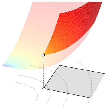
Consider the optimization of a convex function of two variables subject to a box constraint

\[\begin{split} \operatorname*{minimize}_{(x,y)\in\mathbb{R}^2}\quad |x|^3 + y^2 \quad{\rm s.t.}\quad \begin{cases}x\ge1 \\1\le y\le 3.\end{cases} \end{split}\]

The cost function and the constraint are shown below, along with the optimal solution \((x^*,y^*)=(1,1)\).

5.7.1.1. Numerical resolution

Constrained optimization problems can be difficult to solve in closed form, and their resolution almost invariably requires the use of numerical methods. Projected gradient descent is one of such numerical methods, and allows you to solve a problem in three steps:

• implement the cost function with NumPy operations supported by Autograd,

• implement the projection onto the feasible set defined by the intersection of all constraints,

• select the initial point, the step-size, and the number of iterations.

5.7.1.1.1. Cost function

Let’s start with the first step. In this specific example, the cost function computes the number \(|x|^3 + y^2\) given the values \(x\) and \(y\). Its implementation is a Python function that takes a vector w of length 2, where the element w[0] holds the value \(x\), and the element w[1] holds the value \(y\).

cost_fun = lambda w: np.abs(w[0])**3 + w[1]**2

5.7.1.1.2. Projection

The second step deals with the projection onto the feasible set. Since the latter is defined by a box constraint in this specific example, the projection consists of clipping the value \(x\) to the interval \([1,+\infty[\) and the value \(y\) to the interval \([1,3]\). More details can be found in the section discussing the projection of the box constraint.

Remember that the projection must be implemented as a Python function, so you can use either the lambda keyword or the standard def declaration. Just like before, the function takes a vector w of length 2, where the element w[0] holds the value \(x\), and the element w[1] holds the value \(y\).

projection = lambda w: np.clip(w, a_min=[1, 1], a_max=[np.Inf, 3])

5.7.1.1.3. Execution

The third step involves selecting the initial point, the step-size, and the number of iterations.

init = np.random.rand(2)  # initial point
alpha = 0.1               # step-size
epochs = 50               # number of iterations

You are now ready to run projected gradient descent.

w, history = gradient_descent(cost_fun, init, alpha, epochs, projection)

The figure below animates the process for solving the constrained optimization problem. The white dots mark the sequence of points generated by projected gradient descent. The dashed lines show the trajectory travelled by a gradient step and the following projection. Remark that the convergence plot decreases and eventually flattens. This indicates that the optimization algorithm has converged to the constrained minimum.