5.1. Constraints

A constraint is a mathematical condition that must be satisfied by the variables to an optimization problem. Geometrically speaking, a constraint defines a subset of the search space, composed by all the points respecting the mathematical condition. The intersection of all the constraints of an optimization problem defines the feasible set, among whose points the optimal solution must be found. Putting all together, the mathematical problem of finding a point in the feasible set \(\mathcal{C}\subset \mathbb{R}^N\) attaining the lowest value of the function \(J({\bf w})\) is formally denoted as

\[ \operatorname*{minimize}_{\textbf{w}\in\mathbb{R}^N}\;\; J({\bf w}) \;\;\operatorname{subject to}\;\; {\bf w}\in\mathcal{C}. \]

The inclusion \({\bf w} \in \mathcal{C}\) is the most general way to impose one or more constraints on the variables of an optimization problem. Nonetheless, constraints can be expressed in many different manners, as illustrated in the following.

5.1.1. Examples

Consider the following problem

\[\begin{split} \operatorname*{minimize}_{(x,y)\in\mathbb{R}^2}\quad x^2 + y^4 \quad{\rm s.t.}\quad \begin{cases}x\ge1\\0\le y\le 5.\end{cases} \end{split}\]

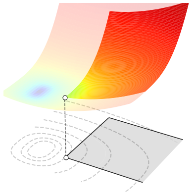
The function to be minimized is \(J(x,y)=x^2 + y^4\). The symbol “s.t.” is short for “subject to” and it is followed by the constraints that the variables must satisfy. According to these constraints, the feasible set \(\mathcal{C}\subset \mathbb{R}^2\) includes all the pairs \((x, y)\) in which the value of \(x\) is at least 1 and the value of \(y\) is between 0 and 5. Although the cost function attains the lowest value at \((0,0)\), this point is not a candidate solution since it does not satisfy the constraints. The optimal solution is actually the pair \((1,0)\), because it is the point with the smallest value of the cost function that satisfies the two constraints. This fact is illustrated in the figure below.

For a more realistic example, suppose you are interested in building a cylindrical can that uses as little material as possible to hold \(V=33\) cm3 of liquid. You are looking for the height \(h\ge0\) and the radius \(r\ge0\) that minimize the surface area \(J(h,r)=2\pi (r^2 + rh)\), but also satisfy the volume constraint \(\pi r^2 h = 33\). This leads to the following problem

\[\begin{split} \operatorname*{minimize}_{(h,r)\in\mathbb{R}^2}\quad 2\pi (r^2 + rh) \quad{\rm s.t.}\quad \begin{cases} \pi r^2 h = 33 \\[0.5em] r\ge0. \end{cases} \end{split}\]

The feasible set \(\mathcal{C}\subset \mathbb{R}^2\) includes all the pairs \((h, r)\) that verify the volume constraint with a positive radius. Note in particular that all the points with \(r\le0\) or \(h\le0\) violate the constraints and thus are unfeasible. Here is another reason why you often have constraints in optimization problems: to avoid solutions that make no sense! The figure below plots the cost function on the feasible set, i.e., the points respecting the constraints. You don’t care what happens elsewhere, because those other points should be never considered as possible candidates to solve your problem. Move the slider to minimize the cost function. The optimal radius is \(r^*=1.74\) cm and the optimal height is \(h^* = 3.48\) cm.

Once Loop Reflect

5.1.2. Common types of constraint

A constraint can be expressed in many different manners, provided that the notation is mathematically sound. But the preferred way is to write them down as inequalities (\(\le, \ge\)) and/or equalities (\(=\)). Depending on its actual definition, a constraint defines a subset that may be empty or nonempty, open or close, convex or nonconvex, and so forth. The following is a brief overview of the most common types of constraint based on their topology. Keep in mind however that such list is very far from being exhaustive.

5.1.2.1. Linear constraint

Linearity is the property of a mathematical relationship that can be graphically represented as a straight line. Linearity plays a big role in mathematics, thanks to its close connection with proportionality. Linear equations and inequalities are also important in constrained optimization, because they can be used to describe many relationships and processes in the physical world. So, in this regard, what is exactly a linear constraint?

A linear constraint is the solution set of linear equalities and inequalities. Formally, this is a subset of \(\mathbb{R}^N\) defined as

\[ \mathcal{C}_{\rm linear} = \big\{ {\bf w} \in \mathbb{R}^{N} \;|\; A' {\bf w} = {\bf b}' \;\;{\rm and}\;\; A'' {\bf w} \le {\bf b}'' \big\}, \]

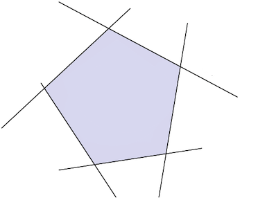
where \(A'\in \mathbb{R}^{K\times N}, A''\in \mathbb{R}^{M\times N}\) and \({\bf b}'\in\mathbb{R}^K, {\bf b}''\in\mathbb{R}^M\). A linear constraint with \(K=0,M=5\) is shown below.

Linear system

Let’s unpack the definition of linear constraint.

• On the one hand, there is a system of \(K\ge0\) linear equalities

\[\begin{split} A' {\bf w} = {\bf b}' \quad\Leftrightarrow\quad \begin{cases} {\bf a}_1'^\top {\bf w} = b_1' \\ \qquad\,\vdots\\ {\bf a}_K'^\top {\bf w} = b_K'. \end{cases} \end{split}\]

• On the other hand, there is a system of \(M\ge0\) linear inequalities

\[\begin{split} A'' {\bf w} \le {\bf b}'' \quad\Leftrightarrow\quad \begin{cases} {\bf a}_1''^\top {\bf w} \le b_1'' \\ \qquad\;\vdots\\ {\bf a}_M''^\top {\bf w} \le b_M''. \end{cases} \end{split}\]

• The set \(\mathcal{C}_{\rm linear}\) consists of the points solving both systems.

The matrices \(A', A''\) and the vectors \({\bf b}', {\bf b}''\) can be freely chosen. However, the corresponding systems must have at least one common solution to ensure that \(\mathcal{C}_{\rm linear}\) is nonempty. Either \(K\) or \(M\) may be zero.

5.1.2.2. Convex constraint

Many relationships cannot be described by linear equations. This is where convexity comes into play, since it is a restricted form of nonlinearity with good mathematical properties. Convexity is probably one of the most important concepts in optimization. If both the cost function and the constraints of an optimization problem are convex, then all minima are guaranteed to be global. This is very convenient for first-order algorithms, because they can only converge to a local minimum by design, like the projected gradient method studied later in this chapter. So, what is a convex constraint anyway?

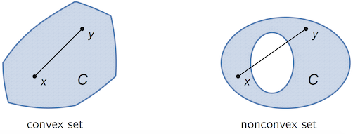
A convex constraint is a subset of \(\mathbb{R}^N\) that, for any pair of points, also contains the line segment connecting them:

\[ \textrm{$\mathcal{C}\subset\mathbb{R}^N$ is convex}\qquad\Leftrightarrow\qquad (\forall {\bf x, y} \in \mathcal{C})(\forall \alpha\in[0,1])\quad \alpha {\bf x} + (1-\alpha){\bf y} \in \mathcal{C}. \]

Intuitively, a convex set is a solid shape with no hollows or indents. Linear constraints are always convex, whereas nonlinear constraints may or may not be convex. An example is given in the figure below.

5.1.2.3. Inequality constraint

We have just seen that constraints can be classified as convex and nonconvex, with linear constraints being an important subcategory of the former. It is also useful to distinguish between equality and inequality constraints. These two classifications can work together to concisely describe constraints. For example, we may refer to convex inequality constraints, nonconvex equality constraints, or any other combination.

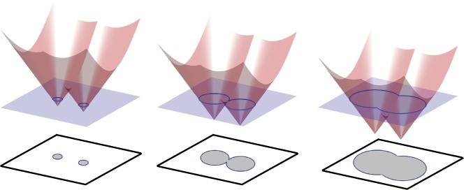
An inequality constraint is the sublevel set of some function \(f\colon\mathbb{R}^N\to\mathbb{R}\), defined as

\[ \mathcal{C}_{\rm sub} = \big\{ {\bf w} \in \mathbb{R}^{N} \;|\; f({\bf w}) \le 0 \big\}. \]

Interestingly, a sublevel set is convex if so is the underlying function:

\[ \textrm{$f$ is convex}\quad\Rightarrow\quad \textrm{$\mathcal{C}_{\rm sub}$ is convex}. \]

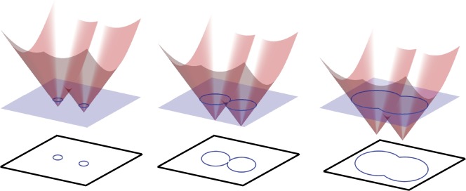
Various examples of sublevel sets are shown in the figure below.

Strict inequalities

Sublevel sets are defined with a not strict inequality in order to include all their boundaries. This is extremely important in constrained optimization, because optimal solutions very often lie on the constraint boundary. Strict inequalities are never used in optimization, except in very specific cases (e.g., with functions defined on open domains, such as \(\log(x)\), \(1/x\), etc…).

5.1.2.4. Equality constraint

An equality constraint is the level set of some function \(h\colon\mathbb{R}^N\to\mathbb{R}\), defined as

\[ \mathcal{C}_{\rm level} = \big\{ {\bf w} \in \mathbb{R}^{N} \;|\; h({\bf w}) = 0 \big\}. \]

An equality constraint defines a subset that contains only the boundary and no interior points. So it is always nonconvex, except when the function \(h\) is affine (in which case it reverts to a linear constraint). This is illustrated in the figure below.

5.1.3. Choosing the right algorithm

The cost function and the constraints determine what is the most appropriate algorithm for solving a constrained optimization problem. When the feasible set is convex, many numerical methods exist for constrained optimization. One such method known as projected gradient descent is studied in this chapter, and it works great with constraints of low to medium complexity. Note however that the task can become considerably more difficult in the presence of “complex” constraints, which often require the use of more advanced optimization methods that are beyond the scope of this chapter.