5.5. Projected gradient descent

Now is the time to answer the fundamental question of this chapter: how to solve a constrained optimization problem? More precisely, the goal is to find a minimum of the function \(J({\bf w})\) on a feasible set \(\mathcal{C}\subset \mathbb{R}^N\), formally denoted as

\[ \operatorname*{minimize}_{{\bf w}\in\mathbb{R}^N}\; J({\bf w}) \quad{\rm s.t.}\quad {\bf w}\in\mathcal{C}. \]

Local optimization methods carry out this task through an iterative process that progressively decreases the cost function while remaining in the feasible set. A simple yet effective way to achieve this goal consists of combining the negative gradient of \(J({\bf w})\) with the orthogonal projection onto \(\mathcal{C}\). This approach leads to the algorithm called projected gradient descent, which is guaranteed to work correctly under the assumption that [1]

• the function \(J({\bf w})\) is Lipschitz differentiable,

• the feasible set \(\mathcal{C}\) is convex.

5.5.1. Algorithm

The necessary optimality condition states that if the point \({\bf w}^\star\) is a minimum of \(J({\bf w})\) on the feasible set \(\mathcal{C}\), then the negative gradient is “orthogonal” to \(\mathcal{C}\) at \({\bf w}^\star\). When the feasible set is convex, such condition can be equivalently expressed using the orthogonal projection (see below for the proof). This yields the following implication, which becomes an equivalence when \(J({\bf w})\) is convex:

\[ \displaystyle{\bf w}^\star \in \operatorname*{Argmin}_{{\bf w}\in\mathcal{C}}\; J({\bf w}) \qquad\implies\qquad {\bf w}^\star = \mathcal{P}_{\mathcal{C}}\big({\bf w}^\star-\alpha\nabla J({\bf w}^\star)\big). \]

The revisited optimality condition motivates an efficient algorithm for constrained optimization. Given an initial point \({\bf w}_0\) and a step-size \(\alpha>0\), the algorithm consists of repeatedly taking a gradient step followed by a projection. The idea is that the gradient step decreases the function value, whereas the projection brings it back onto the feasible set.

Projected gradient descent

\[ {\bf w}_{k+1} = \mathcal{P}_{\mathcal{C}}\big({\bf w}_k - \alpha \nabla J({\bf w}_k)\big) \]

This iterative scheme is illustrated in the figure below for a two-dimensional convex function subject to a box constraint. Moving the slider from left to right animates each step of projected gradient descent. The white dots mark the sequence of iterates \({\bf w}_0, {\bf w}_1, \dots, {\bf w}_k\) generated by the algorithm. The dashed lines show the trajectory travelled by a gradient step \({\bf u}_k = {\bf w}_k - \alpha \nabla J({\bf w}_k)\) and the following projection \({\bf w}_{k+1} = \mathcal{P}_{\mathcal{C}}({\bf u}_k)\). Note the ability of the algorithm to stop at the constrained minimum, once the negative gradient gets “trapped” in the normal cone there.

5.5.1.1. Step size

The projected gradient method is equipped with a step-size. This is a positive value \(\alpha>0\) that controls the distance travelled at each step. Specifically, the distance between two iterates is upper bounded by the gradient magnitude scaled by the step-size. This is easy to prove based on the properties of idempotence \(\big({\bf w}\in\mathcal{C}\;\Rightarrow\;\mathcal{P}_{\mathcal{C}}({\bf w}) = {\bf w}\big)\) and non-expansivity \(\big(\|\mathcal{P}_{\mathcal{C}}({\bf u}) - \mathcal{P}_{\mathcal{C}}({\bf v}) \| \le \|{\bf u} - {\bf v}\|\big)\) held by the projection onto a convex set:

\[\begin{split} \begin{aligned} %\textrm{$\mathcal{C}$ is convex} \quad\Rightarrow\quad \| {\bf w}_{k+1} - {\bf w}_k \| &= \big\| \mathcal{P}_{\mathcal{C}}\big({\bf w}_k - \alpha \nabla J({\bf w}_k)\big) - {\bf w}_k \big\| \\ &= \big\| \mathcal{P}_{\mathcal{C}}\big({\bf w}_k - \alpha \nabla J({\bf w}_k)\big) - \mathcal{P}_{\mathcal{C}}\big({\bf w}_k\big) \big\| \\ &\le \| {\bf w}_k - \alpha \nabla J({\bf w}_k) - {\bf w}_k \| \\ &= \alpha \| \nabla J({\bf w}_k) \|. \end{aligned} \end{split}\]

Recall that the curvature of a Lipschitz-differentiable function is upper bounded by a constant \(L>0\). This guarantees that projected gradient descent converges for any choice of step-size that meets the following condition.

Conservative step-size

\[ \alpha < \frac{2}{L} \qquad {\rm with} \qquad L = \sup_{\mathbf{w}} \; \left\|\nabla^2 J(\mathbf{w})\right\|_2 \]

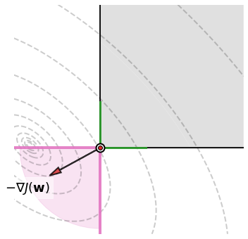
However, this may be a conservative choice, and the preferred approach is to determine a sufficiently small step-size through a trial-and-error strategy guided by the analysis of the convergence plot. If the step-size is chosen correctly, the algorithm will stop at a stationary point of the function \(J({\bf w})\) on the feasible set \(\mathcal{C}\). This arises from the definition of projected gradient descent. Indeed, when the new point \({\bf w}_{k+1}\) does not move significantly from \({\bf w}_k\), it can only mean that the gradient \(-\nabla J({\bf w}_k)\) is either close to zero or nearly orthogonal to \(\mathcal{C}\). The ortogonality is meant in the sense that the negative gradient (red/black arrow) is oriented within the normal cone (pink area). This is by definition a stationary point of \(J({\bf w})\) on \(\mathcal{C}\), in which there exists no feasible descent direction.

Take-away message

• Projected gradient descent converges with a “sufficiently small” step-size.

• The choice of step-size strongly depends on the function to be minimized.

• The reciprocal of the maximum curvature is a conservative upper bound on the step-size.

5.5.1.2. Numerical implementation

Here is the python implementation of projected gradient descent.

def gradient_descent(cost_fun, init, alpha, epochs, project=lambda w: w):
    """
    Finds the minimum of a differentiable function subject to a constraint.
    
    Arguments:
    cost_fun -- cost function | callable that takes 'w' and returns 'J(w)'
    init     -- initial point | array
    alpha    -- step-size     | positive scalar
    epochs   -- n. iterations | integer
    project  -- projection    | callable that takes 'w' and returns 'P(w)'
    
    Returns:
    w       -- minimum point | array with shape equal to the initialization
    history -- cost values   | list of scalars
    """
    
    # Automatic gradient
    from autograd import grad 
    gradient = grad(cost_fun)

    # Initialization
    w = np.array(init, dtype=float)

    # Iterative refinement
    history = []
    for k in range(epochs):
        
        # Projected gradient step
        w = project(w - alpha * gradient(w))
        
        # Bookkeeping
        history.append(cost_fun(w))
        
    return w, history

5.5.2. Proof: Revisiting the optimality condition

The necessary optimality condition states that if the point \({\bf w}^\star\) is a minimum of \(J({\bf w})\) on \(\mathcal{C}\), then the negative gradient is “orthogonal” to \(\mathcal{C}\) at \({\bf w}^\star\). This insight can be formalized by the normal cone, leading to the following implication.

Optimality condition

\[ {\bf w}^\star \in \operatorname*{Argmin}_{{\bf w}\in\mathcal{C}}\; J({\bf w}) \qquad\implies\qquad -\nabla J({\bf w}^\star) \in \mathcal{N}_{\mathcal{C}}({\bf w}^\star) \]

The orthogonal projection is a particular type of constrained optimization problem with \(J({\bf w})=\frac{1}{2}\|{\bf w} - {\bf u}\|^2\). Due to the assumed convexity of the feasible set \(\mathcal{C}\), the optimality condition for the orthogonal projection boils down to

\[ {\bf p} = \mathcal{P}_{\mathcal{C}}({\bf u}) \quad\Leftrightarrow\quad {\bf u}-{\bf p} \in \mathcal{N}_{\mathcal{C}}({\bf p}). \]

Since the normal cone appears in both inclusions, it is possible to rewrite the optimality condition using the orthogonal projection. In this regard, remember that if a vector \({\bf d}\) belongs to the normal cone, then so does the scaled vector \(\alpha{\bf d}\) for every \(\alpha\ge0\). The optimality condition hence stands for any (positively) scaled version of the negative gradient

\[ (\forall\alpha\ge0)\quad -\alpha\nabla J({\bf w}^\star) \in \mathcal{N}_{\mathcal{C}}({\bf w}^\star). \]

Now, add and subtract the optimal solution to the scaled negative gradient

\[ {\bf w}^\star -\alpha\nabla J({\bf w}^\star) - {\bf w}^\star \in \mathcal{N}_{\mathcal{C}}({\bf w}^\star). \]

This new form of optimality condition is exactly the orthogonal projection of the point \({\bf w}^\star -\alpha\nabla J({\bf w}^\star)\) onto the set \(\mathcal{C}\).

Revisited optimality condition (necessary)

\[\begin{split} \begin{cases} \textrm{$\mathcal{C}\,$ is convex} \\[0.5em] \displaystyle{\bf w}^\star \in \operatorname*{Argmin}_{{\bf w}\in\mathcal{C}}\; J({\bf w}) \end{cases} \qquad\implies\qquad {\bf w}^\star = \mathcal{P}_{\mathcal{C}}\big({\bf w}^\star-\alpha\nabla J({\bf w}^\star)\big) \end{split}\]

When \(J({\bf w})\) is convex, this condition is also sufficient.

Revisited optimality condition (sufficient)

\[\begin{split} \begin{cases} \textrm{$J({\bf w})\,$ and $\,\mathcal{C}$ are convex} \\[0.5em] {\bf w}^\star = \mathcal{P}_{\mathcal{C}}\big({\bf w}^\star-\alpha\nabla J({\bf w}^\star)\big) \end{cases} \qquad\implies\qquad {\bf w}^\star \in \operatorname*{Argmin}_{{\bf w}\in\mathcal{C}}\; J({\bf w}) \end{split}\]

The figure below shows the geometric insight behind the revisited optimality condition. The negative gradient (red/black arrow) is “orthogonal” to the constraint at the optimal solution (white dot). The ortogonality is meant in the sense that the negative gradient is oriented within the normal cone (pink area). The picture makes it clear that moving along the negative gradient direction from the optimal solution, one always reachs a point inside the pink area. In turn, the projection of any point in the pink area leads to the optimal solution, because the latter is their closest point that respects the constraint. Both facts can be summarized in one sentence: a projected gradient step taken from the optimal solution leads to the optimal solution itself. This is exactly what says the revisited optimality condition.

5.5.3. Appendix: Nesterov acceleration

Carefully adjusting a constant step-size is the most common approach to make gradient-based methods work. However, if the step-size is too small, the algorithm will converge very slowly, since the steps are too conservative. If the step-size is a little bigger than optimal, the algorithm will converge, but in an oscillatory fashion, overshooting at each iteration. If the step-size is too large, the algorithm diverges.

Ideally, the step-size should be approximately the reciprocal of the second derivative. The problem arises when the second derivative is highly variable. In the one-dimensional case, this could happen for non-quadratic functions, particularly for functions without global bounds on their second derivative. In higher-dimensional settings, the problem could arise from elliptical geometry: the second derivatives are different in different directions, so that it is difficult to choose a step-size that guarantees good convergence in all dimensions. In these cases, one sets a small step-size, obtained as the reciprocal of an upper bound on the global curvature across dimensions (Lipschitz constant of the gradient). It is often harmful to increase the step-size, because doing so might lead the algorithm to diverge along some dimensions, or in some parts of the search space. At the same time, such a small step-size is highly conservative in other parts of the search space. Thus, the problem cannot be remedied by tweaking the step-size.

This is the sort of situation where Nesterov acceleration helps. Nesterov acceleration refers to a general approach that can be used to modify the sequence of points generated by gradient-based methods. The porpuse is to reduce the number of iterations required to reach a stationary point. Intuitively, Nesterov acceleration explores a point near the iterate generated by one step of the algorithm. This exploratory step is governed by an inertial term that depends on the previously explored points. But the beauty of Nesterov method is that despite this exploration, it does not diverge. Even if a particular iteration overshoots the optimum, a few more iterations are enough to get back close to the optimum.

Here is the Nesterov acceleration tailored to projected gradient descent. The idea is to modify the iterate generated by one step of projected gradient step with an exponentially-weighted average of the current and past iterates. The result is an iterative scheme that does no longer ensure to stay in the constraint or to descend on the function at each iteration. It is a small inconvenience to pay for the benefit of enjoying an accelerated convergence.

\[\begin{split} \left\lfloor \begin{aligned} {\bf v}_{k+1} &= \mathcal{P}_{\mathcal{C}}\big({\bf w}_k - \alpha \nabla J({\bf w}_k)\big) \\ {\bf w}_{k+1} &= {\bf v}_{k+1} + \frac{k}{k+3} ({\bf v}_{k+1} - {\bf v}_{k}) \end{aligned} \right. \end{split}\]

This iterative scheme is illustrated below for a two-dimensional convex function subject to the box constraint. Moving the slider from left to right animates each step of projected gradient descent with Nesterov acceleration. The white dots mark the sequence of iterates \({\bf w}_0, {\bf w}_1, \dots, {\bf w}_k\) generated by the algorithm. The dashed lines show the trajectory travelled by one gradient step and the following acceleration that comes after the projection. Note the ability of the algorithm to make longer steps than the non-accelerated version. This allows the accelerated algorithm to reach the constrained minimum in less iterations, although a few more iterations are needed to recover from initially overshooting the constrained minimum. Just like before, the algorithm stops once the negative gradient gets “trapped” in the normal cone there.

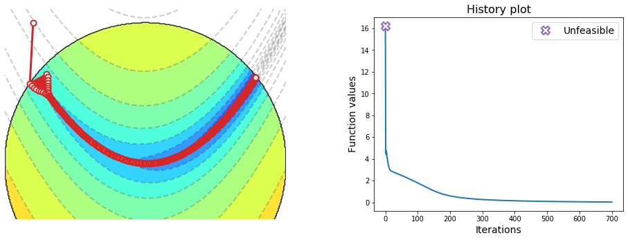
Consider the minimization of the Rosenbrock function subject to the L2-ball:

\[ \operatorname*{minimize}_{{\bf w}\in\mathbb{R}^2}\quad (a - w_1)^2 + b \big(w_2 - w_1^2\big)^2 \quad{\rm s.t.}\quad \|{\bf w}\|\le 1. \]

The Rosenbrock function is notoriously difficult to minimize with gradient-based methods. The global minimum is inside a long, narrow, parabolic shaped flat valley. Finding the valley is trivial, but converging to the global minimum is difficult, because the gradient magnitude is very small inside the valley. The function absolute minimum is \((a, a^2)\), where the parameters are usually set such that \(a=1\) and \(b=100\). Only in the trivial case where \(a=0\) the function is symmetric and the absolute minimum is at the origin. Adding a constraint may obviously change the solution. This happens in the problem considered above, whose solution is no longer \((a, a^2)\), but lies on the boundary of the unit-radius circle.

The figure below illustrates the sequence of points generated by projected gradient descent. The algorithm requires a small step-size, because the gradient magnitude is large outside the valley. However, this leads to a slow progress inside the valley, where the gradient magnitude is small. The algorithm thereby needs several hundred iterations to converge.

rosenbrock = lambda w: (1 - w[0])**2 + 100 * (w[1] - w[0]**2)**2
l2_ball    = lambda w: w * np.minimum(1, 1 / np.linalg.norm(w))

w = gradient_descent(rosenbrock, init=[-0.8,1], alpha=0.003, epochs=700, project=l2_ball)

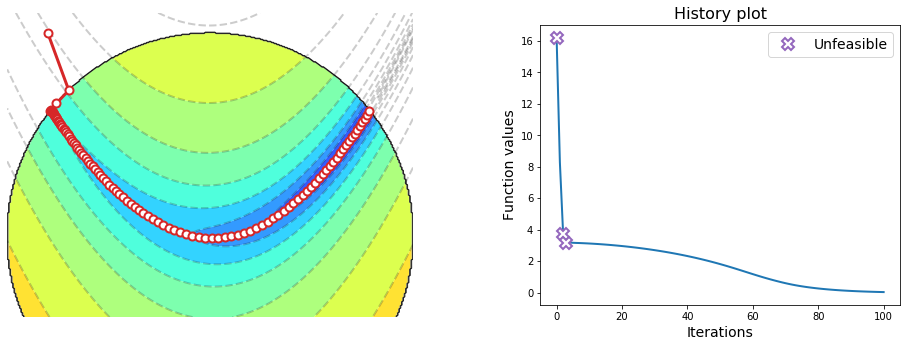
The figure below illustrates the sequence of points generated by projected gradient descent with Nesterov acceleration. Despite the algorithm requires an even smaller step-size, it conveges in only a hundred iterations, scoring an impressive 7x speedup with respect to the non-accelerated version.

init = [-0.8,1]

w = gradient_descent(rosenbrock, init, alpha=0.001, epochs=100, project=l2_ball, nesterov=True)

Here is the python implementation of projected gradient descent with Nesterov acceleration and adaptive restart.

def gradient_descent(cost_fun, init, alpha, epochs, project=lambda w: w, nesterov=False):
    """
    Finds the minimum of a differentiable function subject to a constraint.
    
    Arguments:
    cost_fun -- cost function | callable that takes 'w' and returns 'J(w)'
    init     -- initial point | array
    alpha    -- step-size     | positive scalar
    epochs   -- n. iterations | integer
    project  -- projection    | callable that takes 'w' and returns 'P(w)'
    nesterov -- acceleration  | boolean to activate the acceleration
    
    Returns:
    w       -- minimum point | array with shape equal to the initialization
    history -- cost values   | list of scalars
    """
    
    # Automatic gradient
    from autograd import grad 
    gradient = grad(cost_fun)

    # Initialization
    w = np.array(init, dtype=float)
    v = 0
    k = 0

    # Iterative refinement
    history = []
    for _ in range(epochs):
        
        # Projected gradient step
        u = v
        g = gradient(w)
        v = project(w - alpha * g)
        
        # Adaptive restart
        if nesterov and g @ (v - u) <= 0:
            k = k + 1
        else:
            k = 1
            
        # Nesterov acceleration
        w = v + (k-1)/(k+2) * (v - u)

        # Tracking
        history.append(cost_fun(w))

    return w, history

---

[1]

The algorithm also works with nonconvex constraints if the overall criterion satisfies the Kurdyka-Lojasiewicz property.