6.1. Step-by-step guide

There are always two distinct stages to completely solve an optimization problem.

• Stage 1 - Write down the optimization problem. Based on the given description, you must first formulate the optimization problem, where the variables, the objective function, and possibly some constraints are clearly identified and expressed in formulas.

• Stage 2 - Solve the optimization problem. You can then maximize or minimize the function you wrote down, subject to the constraints you possibly identified. To find the solution, you will use calculus and/or the gradient descent method.

To illustrate these two stages, you will be guided through the solution of several optimization problems.

6.1.1. Unconstrained optimization

Problem. A particle must move from the initial point \((0,0)\) to the final point \((4,2.5)\) crossing three layers of fluids having different densities. The particle travels at speed \(v_1=1\) in the first layer of height \(h_1=1\), at speed \(v_2=0.5\) in the second layer of height \(h_2=1\), and at speed \(v_3=0.8\) in the third layer of height \(h_3=0.5\). What is the fastest path from the initial point to the final point?

6.1.1.1. Stage 1. Problem formulation

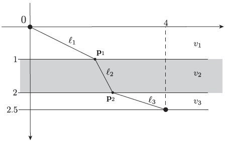
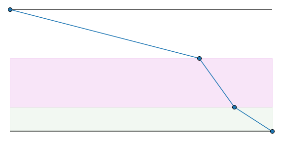
It is always helpful to sketch the described situation. This is when “Stage 1” begins. The picture below shows a possible path that a particle could travel across the three layers. Starting at the origin \({\bf p}_0=(x_0,y_0)=(0,0)\), the particle crosses the first layer at speed \(v_1\) to reach the waypoint \({\bf p}_1 = (x_1, y_1)\) after a stretch of length \(d_1 = \|{\bf p}_1 - {\bf p}_0\|\). The particle then crosses the second layer at speed \(v_2\) to reach the waypoint \({\bf p}_2 = (x_2, y_2)\) after a stretch of length \(d_2 = \|{\bf p}_2 - {\bf p}_1\|\). Finally, the particle reaches the destination \({\bf p}_3=(x_3,y_3)=(4,2.5)\) after a stretch of length \(d_3 = \|{\bf p}_3 - {\bf p}_2\|\).

6.1.1.1.1. Variables

An important decision must be taken now: what are the variables of the problem? Sometimes the variables are clearly stated in the description, but other times the choice is not so obvious. In this example, you may decide to take the horizontal coordinates \(x_1\) and \(x_2\) of the waypoints \({\bf p}_1\) and \({\bf p}_2\) as variables. You don’t need to consider the vertical coordinates, because they are fixed to \(y_1 = h_1=1\) and \(y_2=h_1+h_2=2\) by the problem description. An alternative decision could be to also include the distances \(d_1, d_2, d_3\) among the problem variables, and further introduce the conic constraints \(\|{\bf p}_i - {\bf p}_{i-1}\| \le d_i\) to keep consistency. While both choices have their pros and cons, the first one is easier to deal with. So, the optimization problem will be formulated with respect to the scalar variables \(x_1\) and \(x_2\) representing the horizontal coordinates of the two waypoints.

6.1.1.1.2. Objective function

The next step is to write down a formula for the quantity you want to optimize. Most frequently you’ll use your everyday knowledge of maths, physics, and geometry for this step. In the current example, you are asked to minimize the time needed to travel across the path \({\bf p}_0 \to {\bf p}_1 \to {\bf p}_2 \to {\bf p}_3\). The length of each path section can be expressed in terms of the horizontal positions \(x_1\) and \(x_2\) as follows.

\[\begin{split} \begin{aligned} d_1 &= \|{\bf p}_1 - {\bf p}_0\| = \sqrt{(x_1 - x_0)^2 + (y_1 - y_0)^2} = \sqrt{x_1^2 + 1} \\ d_2 &= \|{\bf p}_2 - {\bf p}_1\| = \sqrt{(x_2 - x_1)^2 + (y_2 - y_1)^2} = \sqrt{(x_2 - x_1)^2 + 1} \\ d_3 &= \|{\bf p}_3 - {\bf p}_2\| = \sqrt{(x_3 - x_2)^2 + (y_3 - y_2)^2} = \sqrt{(4 - x_2)^2 + 0.25} \end{aligned} \end{split}\]

The time for crossing a single layer can be deduced from the definition of speed, which is distance divided by time. So, you can now write a formula for the path-travelling time as a function of the horizontal waypoint positions:

\[\begin{split} \begin{aligned} T(x_1, x_2) &= \frac{d_1}{v_1} + \frac{d_2}{v_2} + \frac{d_3}{v_3}. %\\[0.5em] %&=\sqrt{x_1^2 + 1} + 2 \sqrt{(x_2 - x_1)^2 + 1} + 1.25 \sqrt{(x_2 - 4)^2 + 0.25}. \end{aligned} \end{split}\]

That’s it! You have expressed the quantity you want to optimize in terms of the relevant variables.

6.1.1.1.3. Optimization problem

Putting all together, the optimization problem can be written as

\[ \operatorname*{minimize}_{(x_1,x_2)\in\mathbb{R}^2}\quad \sqrt{x_1^2 + 1} + 2 \sqrt{(x_2 - x_1)^2 + 1} + 1.25 \sqrt{(x_2 - 4)^2 + 0.25}. \]

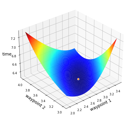
The formulation includes the variables (under the caption “minimize”) and the objective function (after the caption “minimize”). Now, it is always useful to take a moment to double check that the optimization problem is well defined. Let’s plot the objective function to gain a better understanding of the solution. As you can see below, the minimum is located between the values \(2.5\) and \(3.5\) for both variables. Let’s keep going!

6.1.1.2. Stage 2. Problem resolution

Once the optimization problem is clearly formulated, you are ready to start thinking how to solve it. This is when “Stage 2” begins. The first thing to do is to check if the problem can be solved with the analytical approach. The second thing to do is to solve the problem with the numerical approach. In this order preferably.

6.1.1.2.1. Analytical approach

According to the first-order optimality condition, the minimum of a function can be found by computing the partial derivatives with respect to every variable, and setting the resulting expressions to zero. You end up with a system of (possibly nonlinear) equations that may or may not be solved by hand. The answer is likely negative for the current example.

\[\begin{split} \begin{cases} \dfrac{\partial T(x_1, x_2)}{\partial x_1} = 0 \\[0.5em] \dfrac{\partial T(x_1, x_2)}{\partial x_2} = 0 \end{cases} \quad\Leftrightarrow\quad \begin{cases} \dfrac{x_1}{\sqrt{x_1^2 + 1}} + \dfrac{2(x_1 - x_2)}{\sqrt{(x_2 - x_1)^2 + 1}} = 0 \\[0.5em] \dfrac{2(x_2 - x_1)}{\sqrt{(x_2 - x_1)^2 + 1}} + \dfrac{1.25 (x_2 - 4)}{\sqrt{(x_2 - 4)^2 + 0.25}} = 0 \end{cases} %\quad\Leftrightarrow\quad %\begin{cases} %2x_1\sqrt{(x_2 - x_1)^2 + 1} + 4(x_1 - x_2)\sqrt{x_1^2 + 1} = 0 %\\ %4(x_2 - x_1)\sqrt{(x_2 - 4)^2 + 0.25}+ 2.5 (x_2 - 4) \sqrt{(x_2 - x_1)^2 + 1} = 0 %\end{cases} \end{split}\]

6.1.1.2.2. Numerical approach

When the problem is formulated without any constraint, the minimum can be found by the gradient method. The Python implementation of this numerical method requires you to provide the following things:

• the objective function implemented with Numpy operations supported by Autograd,

• the initialization,

• the step-size and the number of iterations.

6.1.1.2.3. Objective function

Let’s start with the objective function. The implementation consists of a Python function that takes one input. Remember: no more than one input argument! The latter is an array with the same shape as the initialization passed to the function gradient_descent. Since the problem has two variables, the initialization will be a vector w of length 2, where the element w[0] holds the variable \(x_1\), and the element w[1] holds the variable \(x_2\). With this convention in mind, here is the Python implementation of the objective function.

def function(w):
    x1 = w[0]
    x2 = w[1]
    cost = np.sqrt(x1**2 + 1) + 2 * np.sqrt((x2 - x1)**2 + 1) + 1.25 * np.sqrt((x2 - 4)**2 + 0.25)
    return cost

Warning

Not everything works with Autograd. Here are the operations that you must avoid in the objective function.

---

• Don’t use assignment to arrays: A[0,0] = x

  • Create new arrays through vectorized operations!

---

• Don’t create lists: u = [x, y]

  • Use arrays: u = np.array([x, y])

---

• Don’t operate on lists: s = np.sum([x, y])

  • Use arrays: s = np.sum(np.array([x, y]))

---

• Don’t use in-place operations: a += b

  • Use binary operations: a = a + b

---

• Don’t use the operation A.dot(B)

  • Use this: A @ B

---

• Never execute the line import numpy as np

  • Use this: import autograd.numpy as np

6.1.1.2.4. Initialization

Let’s move to the initialization. As the optimization problem has 2 variables, the objective function implemented earlier expects a vector of length 2 as input. So your initialization must be a vector of lenght 2. You can manually create a list, which will be internally converted to a float array by the function gradient_descent.

variables = [0, 0]  # list with as many values as the problem variables

Alternatively, you can simply create a random array of appropriate shape. You are free to use any number of axis, as long as you pick a convention and you are consistent with it in the objective function.

variables = np.random.rand(2)  # array with the shape expected by the cost function

6.1.1.2.5. Execution

Now it remains to choose the step-size, set the number of iterations, and run gradient descent.

alpha = 0.5    # step-size
epochs = 100   # number of iterations

w, history = gradient_descent(function, variables, alpha, epochs)

w: [2.88660376 3.42265644]

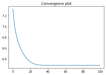
It is always recommended to inspect the convergence plot. Make sure that the curve decreases and eventually gets flat! Otherwise, gradient descent did not converge, and in such case you must go back and try again with different values for the step-size (alpha) and/or the number of iterations (epochs). If the algorithm still does not work, there is probably an issue in the cost function, and you must go back to fix it. Don’t look at the numerical solution before gradient descent has converged!

Tip

Here’s what you can do to make sure that gradient descent converges.

• If the convergence plot skyrockets or a numerical error occurrs (overflow, inf, nan), the step-size is likely too large. Try again by lowering the value assigned to alpha.

• If the convergence plot does not flatten out, the step-size is likely too small. Try again by raising the value assigned to alpha.

• If you cannot increase the step-size without causing numerical errors, but the convergence plot still does not flatten, the algorithm needs more iterations to converge. Try again by raising the value assigned to epochs.

Now the most pleasing part: let’s take a look at the solution!

6.1.2. Optimization with an equality constraint

Problem. You want to construct a window composed of three sections. The middle section is a rectangle, whereas the top and the bottom sections are semi-circles. Given 50 meters of framing material, what are the dimensions of the window that will let in the most light?

6.1.2.1. Stage 1. Problem formulation

Let’s start by sketching the described situation. The window’s shape is shown in the picture below, where the height of the middle rectangle is denoted by the variable \(h\), and the radius of the top/bottom semi-circles is denoted by the variable \(r\). Excellent! You have identified the variables of the problem.

6.1.2.1.1. Objective function

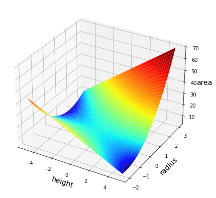
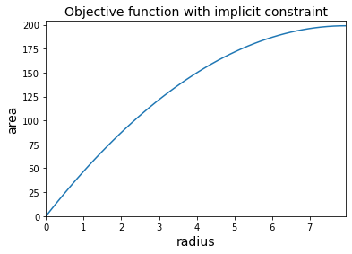
The next step is to write down a formula for the quantity you want to optimize. In the current example, you are asked to maximize the amount of light being let in. This means that you are looking for the values of \(h\) and \(r\) that maximize the window’s enclosed area. So, you now write a formula for the window’s area as a function of the height and the radius:

\[\begin{split} \begin{aligned} A(r, h) &= A_{\rm top} + A_{\rm middle} + A_{\rm bottom} \\ &= \frac{1}{2} \pi r^2 + 2r h + \frac{1}{2}\pi r^2 \\ &= \pi r^2 + 2rh. \end{aligned} \end{split}\]

That’s it! You have expressed the quantity you want to optimize in terms of the relevant variables. Now, it is always useful to take a moment to analyze the function you just defined. Let’s plot the objective function to gain a better understanding of the problem. As you can see below, the window’s area grows more quickly by increasing the radius rather than the height, provided that these quantities are non-negative.

6.1.2.1.2. Equality constraint

Recall that you are given 50 meters of framing material to build the perimeter of the window. So, you now write an equation for the window’s perimeter as a function of the height and the radius:

\[ P_{\rm top} + P_{\rm middle} + P_{\rm bottom} = 50 \quad\iff\quad \pi r + 2h + \pi r = 50 \quad\iff\quad \pi r + h = 25. \]

This is the condition that the height and the radius must satisfy to be considered as possible solutions to the problem.

6.1.2.1.3. Optimization problem

Putting all together, the optimization problem can be written as

\[\begin{split} \operatorname*{maximize}_{(h,r)\in\mathbb{R}^2}\quad \pi r^2 + 2rh \quad\textrm{subject to}\quad \begin{cases} \pi r + h = 25\\[0.5em] r\ge0,\, h\ge0. \end{cases} \end{split}\]

The formulation includes three terms.

• The variables of the problem. These are the height \(h\) and the radius \(r\). They appear under the caption “maximize”.

• The function to be optimized. This is the formula \(\pi r^2 + 2rh\) expressing the window’s area as a function of the height \(h\) and the radius \(r\). It comes after the caption “maximize”.

• The constraints that the optimal solution must satisfy. The equation \(\pi r + h = 25\) states that the window’s perimeter must be exactly \(50\) meters. The inequalities \(\ge0\) further indicate that the height and the radius cannot take negative values. They come after the caption “subject to”.

The optimal solution is the point attaining the largest value of the objective function, among all and only the points satisfying the constraints. The figure below plots the objective function on the points respecting the constraints. You don’t care what happens elsewhere, because the other points cannot be considered as possible candidates to solve the problem.

6.1.2.2. Stage 2. Problem resolution

You are now ready to start thinking how to solve the optimization problem. The major difficulty in your current formulation is given by the equality constraint. You have two options here.

• Try to remove the constraint with a variable substitution. You can only do this if you have an equality constraint that defines an implicit function. In a nutshell, you should be able to manipulate the equality, so that one variable can be expressed as an injective function of the other variables. Otherwise this option is ruled out.

• Use projected gradient descent to directly solve the constrained optimization problem. You can only do this if you can compute the orthogonal projection onto the feasible set. A short list is available in the course notes.

In this specific example, the first option is easier to pursue.

6.1.2.2.1. Remove the equality constraint

The points satisfying the equality constraint form a line where each radius \(r\) is mapped to a unique height \(h\). This happens because the equation implictly defines the height as a function of the radius. There is a little trick to deal with such equality constraints. You can rewrite the equation so that one variable is expressed in terms of the others

\[ \pi r + h = 25 \qquad\iff\qquad h = 25 - \pi r. \]

This is a one-to-one mapping between the radius and the height, in the sense that every value \(h\) is associated to a unique value \(r\) and vice versa. Therefore, you can substitute the variable \(h(r) = 25 - \pi r\) in the objective function

\[ A\big(r, h(r)\big) = \pi r^2 + 2r (25 - \pi r) = 50 r - \pi r^2. \]

The catch is that you must also substitute the variable \(h(r)\) in any other constraint enforced to the original problem. So, the constraint that the height must be non-negative translates into an additional constraint on the radius, that is

\[ h(r) \ge 0 \qquad\iff\qquad 25 - \pi r \ge 0 \qquad\iff\qquad r \le \frac{25}{\pi}. \]

This leads to an equivalent optimization problem that involves only the variable \(r\) over a compact interval

\[ \operatorname*{maximize}_{r\in\mathbb{R}}\quad 50 r - \pi r^2 \quad\textrm{subject to}\quad 0 \le r \le \frac{25}{\pi}. \]

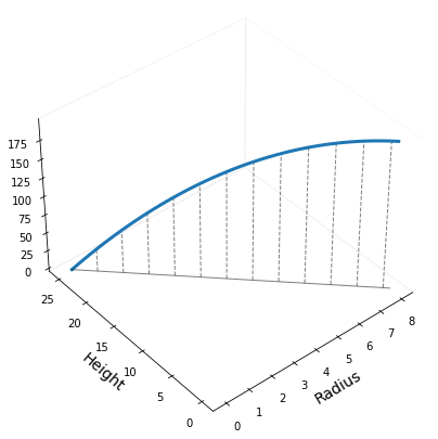
The substitution in the objective function ensures that the equality constraint is implicitly enforced, making it equivalent to the original problem. The reformulated problem is shown in the figure below.

6.1.2.2.2. Analytical approach

Thanks to the substitution trick, you now have an “easier” optimization problem. What comes next is to find the maximum of the function

\[ J(r) = 50 r - \pi r^2. \]

As the function is strongly concave, you can find the unique maximum by setting the derivative to zero, and solving the resulting equation

\[ J'(\bar{r}) = 50 - 2\pi \bar{r} = 0 \quad\iff\quad \bar{r} = \frac{25}{\pi}. \]

The value \(\bar{r}\) belongs the interval \([0, 25/\pi]\), so it is the optimal solution of the transformed problem. The optimal height can be then deduced from the equality constraint, yielding

\[ \bar{h} = 25 - \pi \bar{r} = 0. \]

In conclusion, the optimal window is a circle with radius large enough to use all the framing material.

6.1.2.2.3. Numerical approach

The solution of the transformed problem can be found with the gradient method. This first step is to implement the objective function. This consists of a Python function that takes one input. Such input is a vector of length 1 that contains the variable \(r\). Remark however that the problem aims to maximize the objective function, while gradient descent is designed to minimize a function. You simply need to multiply the function output by \(-1\).

def window_area_implicit(radius):
    area = 50 * radius - np.pi * radius**2
    return -area

The second step is to define the initialization. The problem has one variable, and the cost function implemented earlier expects a vector of length 1 as input. So your initialization must be a vector of lenght 1. You can manually create a list, which will be internally converted to a float array by the function gradient_descent.

init = [0]  # list with as many values as the problem variables

Finally, you can select the step-size, set the number of iterations, and run gradient descent.

alpha = 0.1   # step-size
epochs = 50   # number of iterations

radius, history = gradient_descent(window_area_implicit, init, alpha, epochs)

Radius: [7.95774715]

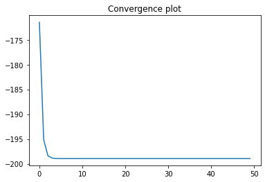
The flattened curve of the convergence plot indicates that the gradient method found the solution. The latter is equal to analytical solution, up to a numerical error. You can thus consider the problem solved!

6.1.3. Optimization with a convex constraint

Problem. A particle must slalom through parallel gates of known position and height. What is the shortest path from the initial position to the final position, using the data given below?

Gate	0	1	2	3	4	5	6
Position	(0,4)	(4,8)	(8,4)	(12,6)	(16,5)	(20,7)	(24,4)
Height		3	2	2	1	1

6.1.3.1. Stage 1. Problem formulation

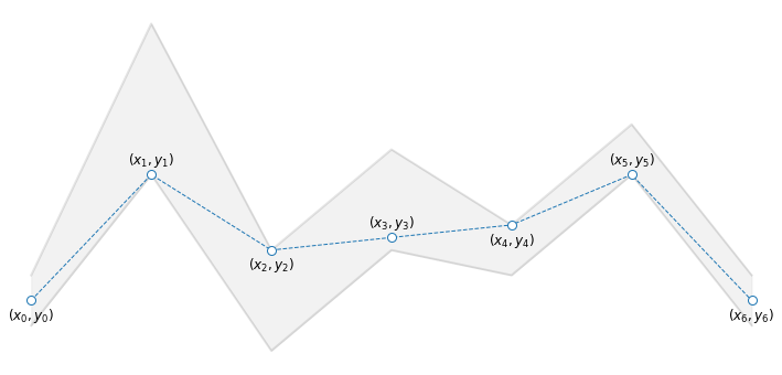
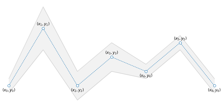
Let’s start by sketching the described situation. The picture below shows a possible path that a particle could travel across the gates. The particle starts at the origin \((x_0,y_0)=(0,4)\), passes through the gates \(n=1,\dots,5\) one after another, and reaches the destination \((x_6,y_6)=(24,4)\). More specifically, the particle crosses the \(n\)-th gate at position \((x_n,y_n)\), traveling a distance \(d_n = \|(x_n,y_n) - (x_{n-1},y_{n-1})\|\) from the previous gate.

6.1.3.1.1. Variables

The problem variables can be the positions \((x_1, y_1), \dots, (x_5, y_5)\) where the particle passes through the gates. You don’t need to consider the origin \((x_0, y_0)\) or the destination \((x_6, y_6)\), because they are fixed by the problem description. Actually, you don’t even need the horizontal coordinates \(x_1, \dots, x_5\), since they are not allowed to move from the markings \(x_n = 4 n\). So, the optimization problem will be formulated with respect to the scalar variables \(y_1, \dots, y_5\) representing the vertical positions where the particle crosses the gates.

6.1.3.1.2. Objective function

You are asked to minimize the distance to travel across the path \((x_0,y_0) \to (x_1,y_1) \to (x_2,y_2) \to (x_3,y_3)\)\(\to (x_4,y_4) \to (x_5,y_5) \to (x_6,y_6)\). The length of each segment can be expressed in terms of the vertical positions as

\[ d_n = \|(x_n,y_n) - (x_{n-1},y_{n-1})\| = \sqrt{16 + (y_n - y_{n-1})^2}. \]

So, you can now write a formula for the total path length as a function of the vertical positions:

\[ D(y_1, y_2, y_3, y_4, y_5) = d_1 + d_2 + d_3 + d_4 + d_5 + d_6. \]

That’s it! You have expressed the quantity you want to optimize in terms of the relevant variables.

6.1.3.1.3. Constraints

Recall that the gates have a predetermined height, and thus the particle must stay inside the limits. In particular, the \(n\)-th vertical position must be within half the height \(h_n\) from the gate vertical center \(c_n\), leading to the box constraint

\[ c_n - \frac{h_n}{2} \le y_n \le c_n + \frac{h_n}{2}. \]

Based on the table provided in the problem description, the constraints on the vertical positions are as follows

\[\begin{split} \begin{cases} 5 \le y_1 \le 11\\ 2 \le y_2 \le 6\\ 4 \le y_3 \le 8\\ 4 \le y_4 \le 6\\ 5 \le y_5 \le 9. \end{cases} \end{split}\]

This is the condition that the vertical positions must satisfy to be considered as possible solutions to the problem.

6.1.3.1.4. Optimization problem

Putting all together, the optimization problem can be written as

\[ \operatorname*{minimize}_{(y_1,\dots,y_5)\in\mathbb{R}^5}\quad \sum_{n=1}^6 \sqrt{16 + (y_n - y_{n-1})^2} \quad\textrm{subject to}\quad c_n - \frac{h_n}{2} \le y_n \le c_n + \frac{h_n}{2} \quad (n=1,\dots,5). \]

The formulation includes three terms.

• The variables of the problem. These are the vertical positions \(y_1,\dots,y_5\). They appear under the caption “minimize”. Note that \(y_0=4\) and \(y_6=4\) are constant.

• The function to be optimized. This is the total length \(d_1+\dots+d_6\) of the particle’s path. It comes after the caption “minimize”.

• The constraints that the optimal solution must satisfy. These are the conditions that the vertical positions must stay within the gate limits \(c_n - h_n/2\) and \(c_n + h_n/2\). They come after the caption “subject to”.

The optimal solution is the point attaining the lowest value of the objective function, among all and only the points satisfying the constraints.

6.1.3.2. Stage 2. Problem resolution

You are now ready to solve the optimization problem. Note that the formulation includes a series of inequalities. These constraints cannot be removed by a change of variables, or by any other kind of manipulation. The only option for solving this optimization problem is to use the projected gradient method, which requires you to provide the following things:

• the objective function,

• the projection onto the feasible set,

• the initialization,

• the step-size, and the number of iterations.

6.1.3.2.1. Objective function

The first step is to implement the objective function. This is a Python function that takes one input. Since the problem has five variables, the input is a vector of length 5, where the first element holds the variable \(y_1\), the second element holds the variable \(y_2\), and so forth. With this convention in mind, here is the Python implementation of the objective function. In general, it is preferable to use vectorized operations, because they are fully supported by Autograd. Special care must be taken if you decide to use loops. See above for the list of operations that must be avoided.

def path_length(y):
    """The input 'y' holds the variables y1, ..., y5."""
    y0 = 4
    y6 = 4
    yext = np.hstack(([y0], y, [y6]))  # Insert y0 and y6 into 'y' before computing the distances
    diff = np.diff(yext)
    dist = np.sqrt(16 + diff**2)
    length = np.sum(dist)
    return length

6.1.3.2.2. Projection

The second step is to implement the projection onto the feasible set. Since the latter is defined by a box constraint, the projection consists of clipping each variable \(y_n\) between the limits \(c_n - \frac{h_n}{2}\) and \(c_n + \frac{h_n}{2}\). More details can be found in the section discussing the projection onto the box constraint. Remember that the projection must be implemented as a Python function that takes a vector as input and returns a vector of the same size as output. Such vector is of length 5, because the problem has five variables. With this convention in mind, here is the Python implementation of the projection.

center = np.array([8, 4, 6, 5, 7])
height = np.array([3, 2, 2, 1, 1])
inf = center - height/2
sup = center + height/2

project = lambda w: np.clip(w, inf, sup)

6.1.3.2.3. Initialization

The third step is to define the initialization. As the optimization problem has 5 variables, the objective function and the projection implemented earlier expect a vector of length 5 as input. So your initialization must be a vector of lenght 5.

init = np.zeros(5)

6.1.3.2.4. Execution

The final step is to select the step-size, set the number of iterations, and run gradient descent.

alpha = 1      # step-size
epochs = 50   # number of iterations

y, history = gradient_descent(path_length, init, alpha, epochs, project)

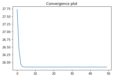
The flattened curve of the convergence plot indicates that the gradient method found the solution. Watch out that sometimes the curve looks flat, but it is still slowly decreasing. So it is better to not cheap out on the iterations. Now the most satisfyinng part: let’s take a look at the solution!