Variable step-size

The common practice when using gradient descent is to choose a constant step-size (usually by trial and error) that induces the most rapid convergence to a stationary point. This often means aiming at the largest possible value that leads to proper convergence. The advantage of picking a large step-size is that gradient descent can reach lower values of the function being optimized in as few iterations as possible. But if the step-size is too large, gradient descent oscillates and fails to converge to a stationary point. To circumvent this issue, a simple yet effective strategy is to slowly diminish the step-size during the optimization process in accordance to a predetermined schedule. The sequence generated by gradient descent thus becomes the following

\[ \textbf{w}_{k+1} = \textbf{w}_k - \alpha_k \nabla J(\textbf{w}_k), \]

where the step-size \(\alpha_k\) shrinks as the iteration number \(k\) increases, instead of remaining constant. By doing so, gradient descent can start with a larger step-size to quickly locate a minimum, and finish with a smaller step-size to ensure a proper convergence. This technique known as step-size scheduling may prove useful in several situations.

• When a function is differentiable almost everywhere, a diminishing step-size is absolutely necessary. This is because the optimization process oscillates and never converges if the gradient is discontinuous at a stationary point.

• When a function is nonconvex, a diminishing step-size may be beneficial to achieve faster convergence, prevent oscillations, and escape undesirable local minima. This is because large steps are more likely to accelerate convergence and escape undesirable local minima, whereas small steps are more suitable to damp oscillations and ensure proper convergence to a nearby stationary point. A diminishing step-size combines both strategies organically, in the hope that larger steps drive the optimization process toward a global minimum (or a good local minimum), before smaller steps kick in to eventually achieve the convergence.

Scheduling

Schedules define how the step-size changes over the time when gradient descent is running, and are typically specified for each iteration. This is mainly done by setting additional decay parameters beforehand, without using any feedback throughout the optimization process. The following are some of the most popular schedules.

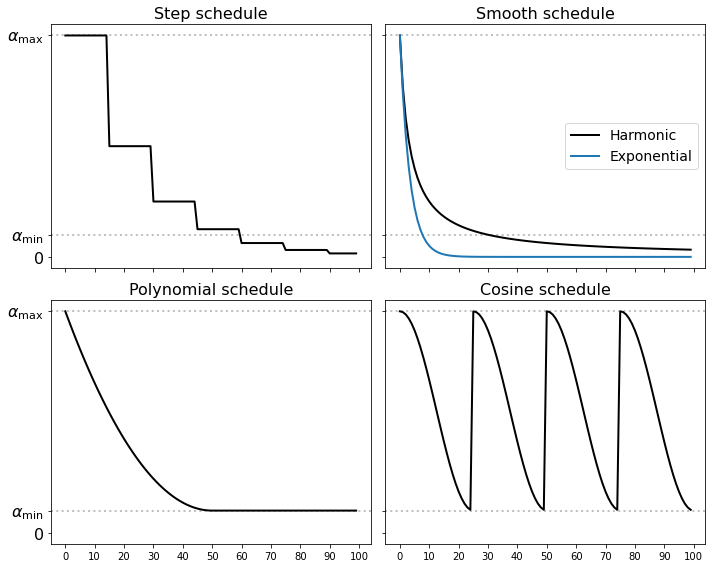
• Step decay. The step-size is reduced by a factor \(0<c<1\) every \(r\) iterations, according to the formula

\[ \alpha_k = \alpha_\max \, c^{\left\lfloor(1+k)/r\right\rfloor}. \]

• Harmonic decay. The step-size follows an harmonic progression with factor \(d>0\), according to the formula

\[ \alpha_k = \frac{\alpha_\max}{1+dk}. \]

• Exponential decay. The step-size is smoothly reduced by an exponential factor \(d>0\), according to the formula

\[ \alpha_k = \alpha_\max \, e^{-dk}. \]

The above schedules shrink the step-size to zero as the number \(k\) of iterations goes to infinity. The beauty of this choice is that there is no limit to total traveled distance, since the sum \(\alpha_0 + \alpha_1 + \dots+\alpha_k + \dots\) is unbounded. In practice however, it could happen that the step-size becomes too small after a certain number of iterations, slowing down the convergence considerably. The following schedules counter this issue by introducing a lower bound on the the step-size.

• Polynomial decay. The step-size starts from \(\alpha_\max\) and smoothly reduces to \(\alpha_\min\) with rate \(p\ge1\) over the first \(r\) iterations, according to the formula

\[\begin{split} \alpha_k = %\begin{cases} %\alpha_\min & \textrm{if $k > r$}\\ \alpha_\min + \big(\alpha_\max - \alpha_\min\big) \max\big(0,1 - \dfrac{k}{r}\big)^p. %& \textrm{otherwise}. %\end{cases} \end{split}\]

• Cosine annealing. The step-size is cyclically reduced from \(\alpha_\max\) to \(\alpha_\min\) every \(r\) iterations, according to the formula

\[ \alpha_k = \alpha_\min + \frac{1}{2}\big(\alpha_\max - \alpha_\min\big) \Big(1 + \cos\big(\pi \, k/r-\pi\left\lfloor k/r\right\rfloor\big)\Big). \]

The different schedules are shown below. In all cases, they require to manually choose the step-size and the decay parameters, whose optimal values can vary greatly depending on the optimization problem at hand. Moreover, a cyclic schedule such as the cosine annealing requires to keep track of the best minimum seen so far in the optimization process (i.e., the one providing the lowest function value), because the final point resulting from a run may not provide the lowest value.

Almost-everywhere differentiability

Gradient descent relies on the hypothesis that the function being optimized is Lipschitz differentiable. This ensures that the gradient shrinks gradually to zero while approaching a stationary point, which ultimately is the reason why the algorithm converges with a sufficiently small step-size. But what happens if a function is differentiable almost everywhere? For example, consider the function

\[ J(w) = |w| \]

whose derivative is defined everywhere but in \(w=0\) as

\[\begin{split} J'(w) = \begin{cases} +1 &\textrm{if $w>0$}\\ -1 &\textrm{if $w<0$}. \end{cases}\end{split}\]

Remark that the derivative has a jump discontinuity in \(w=0\). Unfortunately, such discontinuity precludes the gradient method from working properly. The difficulty stems from the fact that the derivative does not vanishes at the minimum. This causes pathological oscillations that prevent the convergence regardless of how small the step-size has been chosen. The phenomenon is illustrated in the animation below. Note that the convergence plot never gets flat.

Step-size scheduling is the simplest fix to deal with functions that are differentiable almost everywhere. In particular, a diminishing step-size is absolutely necessary to damp oscillations caused by discontinuities in the gradient. The animation below runs the gradient method with a step-size that decays according to the following schedule

\[ \alpha_k = \frac{\alpha}{1+k}. \]

The above step-size clearly decreases to zero as the algorithm goes. The beauty of this choice is that the total traveled distance goes to infinity. So in theory an algorithm employing this schedule can move an infinite distance in search of a minimum while taking smaller and smaller steps, so as to work into any “small nooks and crannies” a function might have where any minimum lie. This can be clearly seen below.

Nonconvexity

Step-size scheduling can be especially effective with nonconvex functions, even when they are Lipscitz differentiable. In nonconvex settings, it is usually better to take large steps at the beginning of the optimization process, because they are more likely to help escape local minima. However, large steps prevent the algorithm from converging to a stationary point. This issue can be circumvented by diminishing the step-size during the optimization process. By doing so, gradient descent starts with larger step-sizes to hopefully reach the valley of a global minimum (or a good local minimum), and then gradually switches to smaller step-sizes to properly converge to a nearby stationary point.

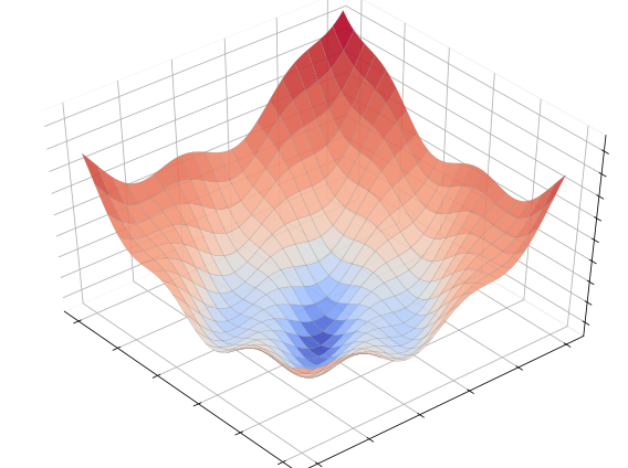
Let’s explore this idea in pictures by considering the nonconvex optimization problem

\[ \operatorname*{minimize}_{{\bf w}\in\mathbb{R}^2}\quad \frac{1}{2}\|{\bf w}\|^2 + 2\sin(1.5w_1 + 1.5w_2)^2. \]

The cost function is displayed below. Note the presence of a global minimum surrounded by two local minima.

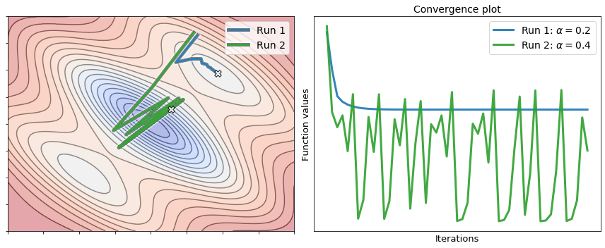
The next figure shows two runs of gradient descent to minimize the above function. The first run uses a small step-size, whereas the second run uses a larger step-size. It is interesting to analyze their behavior by looking at the convergence plot. The first run (small step-size) achieves a descent at each iteration, but it merely converges to a local minimum. Conversely, while the second run (large step-size) oscillates wildly and never comes to a stop, it escapes the local minimum and reaches the valley where the global minimum is located.

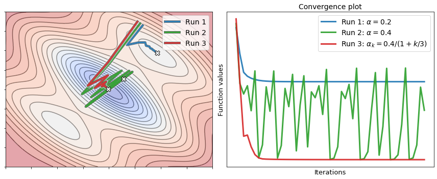
The figure below shows a third run of gradient descent with a large step-size that decays according to the following schedule

\[ \alpha_k = \frac{\alpha}{1+k/3} \]

with \(\alpha=0.4\). Interestingly, this run escapes the local minimum and converges to the global minimum. The reason is that the steps taken by the algorithm are large at the beginning, but they become smaller and smaller as the iterations go by.