2.1. Optimization problem

Optimization is the problem of selecting the best element with respect to some criterion. In the simplest case, an optimization problem consists of maximizing or minimizing a function within an allowed set of available alternatives. Optimization can be divided into two categories, depending on whether the variables are continuous or discrete. This course focuses exclusively on continuous optimization, in which an optimal value from a continuous function must be found, and the seeked solution is expressed as a vector of real numbers. Because of this assumption, continuous optimization allows the use of calculus techniques. An example of continuous optimization is presented in the following.

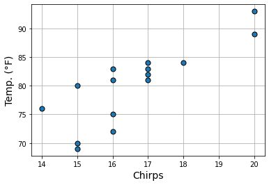
2.1.1. Example: Cricket chirps

Did you know that you can estimate the temperature by listening to the rate of cricket chirps? The following figure shows measurements of the number of chirps (over 15 seconds) of a striped ground cricket at different temperatures measured in degrees Farenheit. The plot indicates that the measured quantities are roughly correlated: the higher the temperature, the faster the cricket chirps.

Measurements

Chirps	20	16	20	18	17	16	15	17	15	16	15	17	16	17	14
Temp (°F)	89	72	93	84	81	75	70	82	69	83	80	83	81	84	76

2.1.2. Linear model

You are interested in finding the line that best approximates the relationship between the cricket chirps and the temperature. Mathematically, a line can be expressed via the simple formula

\[ {\sf temperature} = a \cdot {\sf chirps} + b. \]

Therefore, the task of fitting a line to some points is equivalent to the problem of estimating the slope \(a\) and the intercept \(b\). The animation below shows that it is possible to represent any line by changing the slope \(a\) and intercept \(b\). Move the slider to interact with the plot.

2.1.3. Mathematical formulation

The \(P=15\) measurements can be represented as a set of two-dimensional points

\[\mathcal{S} = \big\{ (x_p,y_p) \in \mathbb{R}^2 \;|\; p=1,\dots,P\big\},\]

where each measurement is denoted by a point \((x_p,y_p)\) such that

• \(x_p\) = cricket chirps,

• \(y_p\) = temperature (°F).

How to find the line that best fits the measurements? According to the linear model previously defined, one needs to find the parameters \(a\) and \(b\) so that the following approximations hold as tight as possible:

\[\begin{split} \begin{aligned} a x_1 + b &\approx y_1 \\ a x_2 + b &\approx y_2 \\ &\,\,\vdots \\ a x_P + b &\approx y_P. \end{aligned} \end{split}\]

The above statement says that the error between \(a x_p + b\) and \(y_p\) must be small for every \(p\in\{1,\dots,P\}\). A possible way to measure the error between two scalar quantities is to square their difference, namely

\[ (\forall p\in\{1,\dots,P\})\qquad (a x_p + b - y_p)^2 \approx 0. \]

To ensure that all such values are small, one can minimize their average

\[ J(a,b) = \frac{1}{P}\sum_{p=1}^P (a x_p + b - y_p)^2.\]

This is a continuous function that measures how well a line fits the points \((x_1,y_1),(x_2,y_2),\dots,(x_P,y_P)\), given a specific combination of values for the slope \(a\) and the intercept \(b\). Therefore, the “right values” for the parameters \(a\) and \(b\) can be computed by finding the minimum of the function \(J(a,b)\). Such problem is mathematically expressed as

\[ \operatorname*{minimize}_{(a,b) \in \mathbb{R}^2} \; J(a, b). \]

The solution to the above optimization problem is the point \((a^*, b^*)\) that minimizes the mean squared error defined by the function \(J(a,b)\). The animation below illustrates that the optimal values for \(a\) and \(b\) are located at the lowest point of the function. Move the sliders to find the minimum of the function.

2.1.4. Choosing the right algorithm

Inspecting the overall shape of the cost function helps determine what is the most appropriate method for finding the solution of an optimization problem. In the previous example, it is easy to check that the cost function \(J(a,b)\) is convex with respect to the parameters \(a\) and \(b\). Convexity means that the function curvature is always positive. Because of this, we are guaranteed that all the minima of the cost function are globally optimal. Such scenario is indeed very favorable for solving optimization problems with most numerical methods.