2.3. Zero-order optimality

The problem of finding a minimum of the function \(J(\mathbf{w})\) is formally phrased as

\[\operatorname*{minimize}_{\mathbf{w} \in \mathbb{R}^N} \; J(\mathbf{w}).\]

This means looking into every possible point \(\mathbf{w}\) to find one that gives the smallest value \(J(\mathbf{w})\).

2.3.1. Extrema of a function

A point attaining the smallest value of a function is called global minimum.

Global minimum

\[ %{\bf w}^\star_\min\in\mathbb{R}^N %\quad\textrm{such that}\quad (\forall{\bf w}\in\mathbb{R}^N)\quad J({\bf w}^\star_\min) \le J({\bf w}) \]

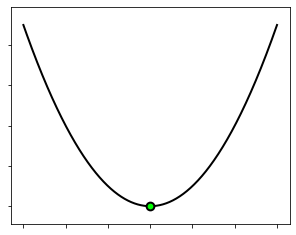
We can attempt to visualize a low-dimensional function (\(N\le2\)) to have a look at its minima. Below is plotted the quadratic function \(J(w)=w^2\), whose global minimum at \(w^*=0\) is marked with a green dot in the figure.

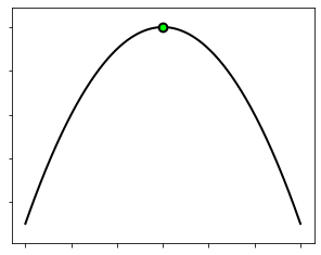
It is interesting to remark what happens if we multiply the quadratic function by \(−1\). The function flips upside down, becomes unbounded from below, and does no longer have any global minima. Now, the point \({w}^* = 0\) turns into a global maximum, which is defined as a point attaining the largest value of the function.

Global maximum

\[ %{\bf w}^\star_\max\in\mathbb{R}^N %\quad\textrm{such that}\quad (\forall{\bf w}\in\mathbb{R}^N)\quad J({\bf w}^\star_\max) \ge J({\bf w}) \]

This is shown in the next figure, where the maximum is marked with a green dot.

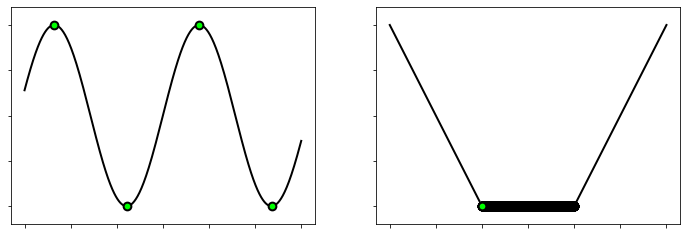
Let us look at the sinusoid function \(J(w) = \sin(2w)\) plotted below (left side). Here, we can clearly see that there are two global minima and two global maxima, marked by green dots, over the range we have plotted the function. We can imagine of course that there are further minima and maxima (here one exists at every \(4k+3\) multiple of \(\pi/2\) for integer \(k\)). So, this is just an example where the function has an infinitely many global minima and maxima. A function may also have infinitely many global minima over a compact subset (right side).

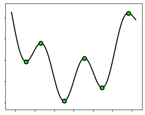
The goal of optimization is to find a point that is globally optimal. This may not always be possible, depending on the “difficulty” inherent to a given function. In such cases, we are forced to settle for a point that is only locally optimal. In this regard, let’s look at the function \(J(w)=\sin(3w)+0.1w^2\) plotted below. Here, we have a global minimum at \(w^* = −0.5\). We also have minima and maxima that are locally optimal, for example the points at \(w' = 0.8\), \(w'' = 1.5\), and \(w''' = 2.7\). We can formally say that a point is a local minimum if it attains the smallest point on the function nearby.

Local minimum

\[ %{\bf \bar{w}}_{\rm local}\in\mathbb{R}^N %\quad\textrm{such that}\quad (\forall{\bf w}\;{\rm near}\; {\bf \bar{w}}_{\rm local})\quad J({\bf \bar{w}}_{\rm local}) \le J({\bf w}) \]

The statement “for all \({\bf w}\) near \({\bf \bar{w}}_{\rm local}\!\)” means that we are only considering the neighboring points of \({\bf \bar{w}}_{\rm local}\). The same formal definition can be made for local maxima by switching \(\le\) with \(\ge\), just as in the case of global minima and maxima.

From these examples, we have seen how to formally define global minima/maxima, as well as the local minima/maxima. These formal definitions directly generalize to a function of any dimension. Packaged together, they are often referred to as the zero-order optimality conditions.

2.3.2. Existence and unicity

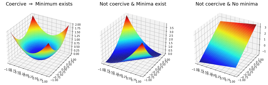
The foremost assumption in optimization is that the function \(J({\bf w})\) must be continuous. This is however not enough to guarantee the existence of a global minimum, since a continuous function may have between zero and an infinite number of minima. One additional requirement is coercivity, so that the function grows to infinity at infinity. The combination of continuity and coercivity ensures the existence of at least one global minimum. [1]

Existence of minima

\[ \textrm{$J({\bf w})$ is continuous and coercive} \quad\Rightarrow\quad \textrm{$J({\bf w})$ has a global minimum} \]

This is a sufficient condition. Some non-coercive functions may still have a global minimum, as shown below.

In optimization, it is very important to distiguish between convex and nonconvex functions. Why? Because convexity allows for better characterizing the minima of a function. One of the most useful facts in optimization is that all the minima of a convex function are global (and constitute a convex set).

Convexity \(\Rightarrow\) globality

\[ \textrm{$J({\bf w})$ is convex}\quad\Rightarrow\quad \textrm{All minima of $J({\bf w})$ are global} \]

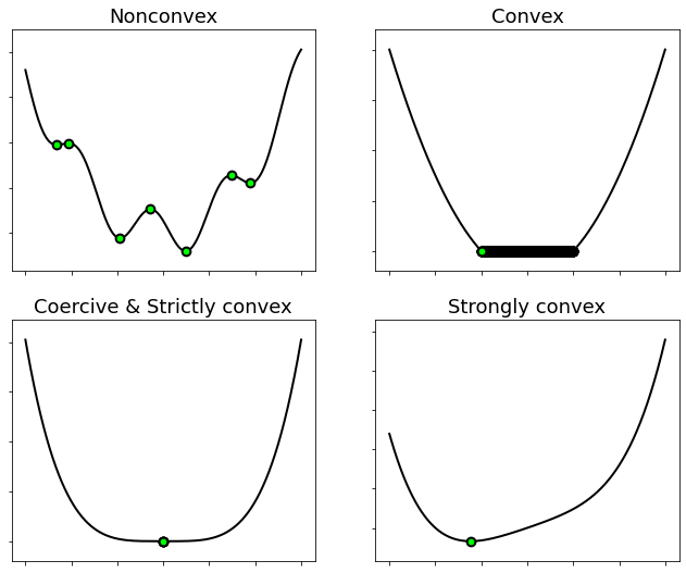
More precisely, the number of minima held by a function depends on its type of convexity.

• Nonconvex \(\Rightarrow\) Zero or any number of global and local minima.

• Convex \(\Rightarrow\) Zero, one, or an infinite number of global minima. No other value is possible.

• Strictly convex \(\Rightarrow\) Zero or one global minimum.

• Strongly convex \(\Rightarrow\) Exactly one global minimum.

• Coercive & Strictly convex \(\Rightarrow\) Exactly one global minimum.

These properties can be intuitively understood by looking at the pictures below.

Note

• A convex function “curves up” without any bends the other way.

  • This includes linear functions as well.

• A strictly convex function has greater curvature than a linear function.

  • Convex functions that do not have linear or flat sections anywhere in their domain are strictly convex.

• A strongly convex function has at least the same curvature as a quadratic term.

  • Adding the squared norm (scaled by some \(\mu>0\)) to a convex function makes it strongly convex.

2.3.3. Equivalent problems

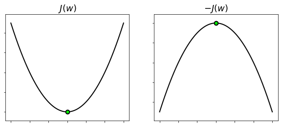
The concepts of minima and maxima of a function are always related to each other via multiplication by \(−1\). Any point that is a minimum of a function \(J({\bf w})\) is also a maximum of the function \(-J({\bf w})\) and vice versa. Therefore, minimizing \(J({\bf w})\) is equivalent to maximizing \(-J({\bf w})\), because the minima of the former coincides with the maxima of the latter.

Equivalence I

\[ \operatorname*{minimize}_{\bf w}\; J({\bf w}) \quad\Leftrightarrow\quad \operatorname*{maximize}_{\bf w}\; -J({\bf w}). \]

Note also that if \(J({\bf w})\) is convex, then \(-J({\bf w})\) is concave. See the figure below.

There is a limited number of operations that preserve the extrema of a function. These operations may be useful to reveal the hidden convexity of an optimization problem, or to make it numerically stable. For exemple, a strictly increasing function \(h\colon\mathbb{R}\to\mathbb{R}\) does not change the (global or local) extrema of a function \(J({\bf w})\), yielding the following equivalence.

Equivalence II

\[\begin{split} \begin{aligned} \operatorname*{minimize}_{\bf w}\; J({\bf w}) \quad\Leftrightarrow\quad &\operatorname*{minimize}_{\bf w}\; h\big(J({\bf w})\big). \\[-1em] &\hphantom{\operatorname*{minimize}_{\bf w}\;}\downarrow \\[-2em] &\quad\;\;\,{\scriptstyle \textrm{(strictly increasing)}} \end{aligned} \end{split}\]

Strictly increasing functions include affine transformations with positive slope, the exponential, the logarithm over \(\mathbb{R}_{++}\), the square root over \(\mathbb{R}_{+}\), the power over \(\mathbb{R}_{+}\), and so forth. See the examples below.

Moreover, a one-to-one mapping \(\phi\colon\mathbb{R}^K\to\mathbb{R}^N\) (also known as injective function ) can be used to change the variables of an optimization problem without modyfing its solutions, leading to the following equivalence.

Equivalence III

\[\begin{split} \begin{aligned} \operatorname*{minimize}_{{\bf w}\in\mathbb{R}^N}\; J({\bf w}) \quad\Leftrightarrow\quad &\operatorname*{minimize}_{{\bf u}\in\mathbb{R}^K}\; J\big(\phi({\bf u})\big). \\[-1em] &\hphantom{\operatorname*{minimize}_{\bf w}\;J\big(}\downarrow \\[-2em] &\qquad\;\;\,{\scriptstyle \textrm{(one-to-one mapping)}} \end{aligned} \end{split}\]

For example, consider a posynomial function

\[ J({\bf w}) = \sum_{k=1}^K \gamma_k w_1^{a_{k,1}}w_2^{a_{k,2}}\dots w_N^{a_{k,N}} \]

with \(\gamma_k>0\) and \(a_{k,n}\in\mathbb{R}\). The change of variables \(w_n = e^{u_n}\) yields

\[\begin{split} \begin{aligned} J(e^{\bf u}) &= \sum_{k=1}^K \gamma_k (e^{u_1})^{a_{k,1}}(e^{u_2})^{a_{k,2}}\dots (e^{u_N})^{a_{k,N}} \\ &= \sum_{k=1}^K \exp\big(\log(\gamma_k) + u_1 a_{k,1} + \dots + u_N a_{k,N}\big) \\ &= \sum_{k=1}^K \exp\big(b_k + {\bf a}_k^\top {\bf u}\big). \end{aligned} \end{split}\]

Since the variable change is given by a one-to-one mapping, a minimum of \(J({\bf w})\) can be computed as \({\bf w}_\min^* = e^{{\bf u}_\min^*}\), where \({\bf u}_\min^*\) is a minimum of the convex function \(J(e^{\bf u})\) with respect to \({\bf u}\).

---

[1]

The result still holds if continuity is replaced by lower semi-continuity.