4.6.4. Example 4

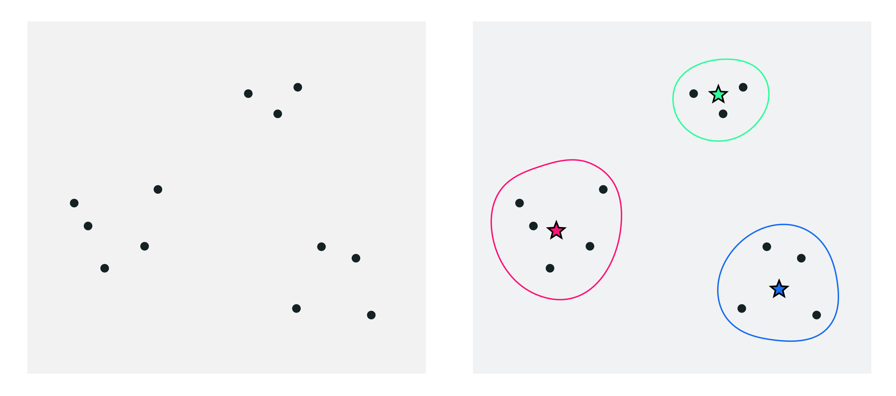
Look at the points shown in the left figure. Notice how they naturally group together in three clusters. The right figure highlights the three clusters (circles) and their centers (stars). The cluster centers are commonly known as centroids. How to regroupe a set of data points into clusters, so that each point belongs to the group with the nearest centroid? The answer is to formulate this task as an optimization problem.

4.6.4.1. Notation

The letter \(P\) indicates the number of points, which are denoted as

\[\textrm{points}\quad\rightarrow\quad {\bf x}_1, {\bf x}_2,\dots,{\bf x}_P. \]

The letter \(K\) denotes the number of clusters. Each cluster has a centroid, which are denoted as

\[\textrm{centroids}\quad\rightarrow\quad {\bf c}_1, {\bf c}_2,\dots,{\bf c}_K. \]

Each point/centroid is a vector of size \(N\). Finally, the indices of the points belonging to the \(k\)-th cluster are denoted as

\[ \mathcal{S}_k = \Big\{p\in\{1,\dots,P\} \;\big|\; \textrm{${\bf x}_p$ belongs to the cluster $k$} \Big\}. \]

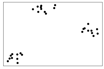
The following is a set of \(P=30\) points with \(N=2\) dimensions grouped in \(K=3\) clusters.

4.6.4.2. Analytical solution

With the notation in hand, the clustering scenario can be described more precisely. In a nutshell, the goal is to find the centroids that “best” represent the given points. It seems intuitive to define the centroids as the average of the points assigned to each cluster. Algebraically this is equivalent to say that

\[ \mathbf{c}_k = \frac{1}{\left\vert\mathcal{S}_k\right\vert}\sum_{p\in\mathcal{S}_k}\mathbf{x}_p. \]

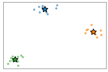
Since the sets \(\mathcal{S}_k\) are unknown in general, this formula cannot be directly used to find the centroids. Nonetheless, it can be used to compute the centroids for the above set of points, as we have generated the data by ourselves, and thus we know all the point-cluster assignments. Here is the expected solution to the problem, which is often referred to as groundtruth.

4.6.4.3. Cost function

To formulate the optimization problem, we can state mathematically an obvious and implicit fact about the clustering scenario. Each point belongs to the cluster with the closest centroid. To express this algebraically, we can say that a point must belong to the cluster whose centroid is at minimal distance. Such distance can be computed as

\[ d_p = \min_{k\in\{1,\dots,K\}}\; \left\Vert \mathbf{x}_p - \mathbf{c}_k \right\Vert^2. \]

To find the centroids that best fit the points, we minimize the above distance for all \(p=1,\dots,P\), yielding the cost function

\[ J(\mathbf{c}_1, \dots, \mathbf{c}_K) = \sum_{p=1}^P\,\min_{k\in\{1,\dots,K\}}\; \left\Vert \mathbf{x}_p - \mathbf{c}_k \right\Vert^2. \]

This is a nonconvex differentiable function that can be optimized with gradient descent.

4.6.4.4. Optimization

The figure below shows the process of gradient descent applied to minimize this function. Since the cost function is too high dimensional to be visualized, the animation focuses on the sequence of cluster centroids generated by gradient descent.

4.6.4.5. Importance of initialization

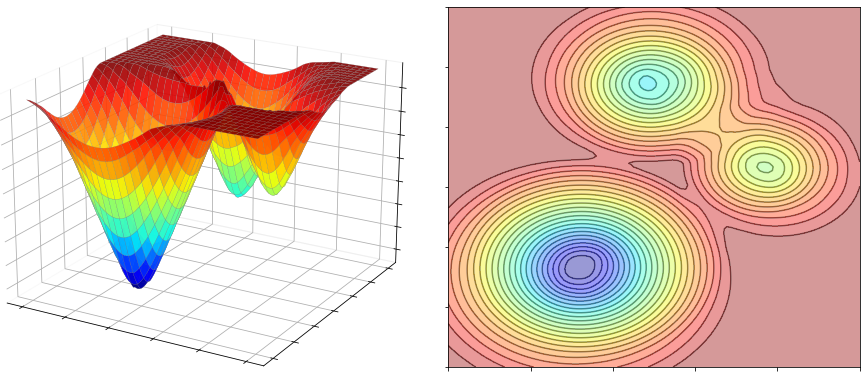
The next figure shows the cost function plotted with respect to one of the centroids. You can see the presence of 3 minima, 3 saddle points, 1 maximum, and a plateau all around. In reality, there are many more stationary points, but they cannot be easily visualized, due to the high dimensionality of the cost function.

Since it is a nonconvex problem, clustering can fail due to a poor choice of the initial centroids. A good initialization is the one where the initial centroids are spread evenly throughout the distribution of the data, as this allows the optimization algorithm to better find good minima. Conversely, a poor initialization is typically the one where all of the initial centroids are bunched up together in a small region of the space. This can make it difficult for the centroids to spread out effectively, leading to a less than optimal clustering.

4.6.4.5.1. Empty clusters

The first issue stemming from a poor initialization is that of empty clusters, where some centroids have no point assigned to them. It is indeed possible for clusters to end up being empty, as illustrated in the animation below.

4.6.4.5.2. Suboptimal clusters

The second issue stemming from a poor initialization is that of suboptimal clusters, where the centroids fail to capture the structure of the data, even though the correct number of clusters is chosen. This is illustrated in the animation below.

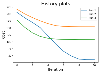
4.6.4.5.3. Restart strategy

The best way to deal with nonconvexity is to run gradient descent multiple times with a different initialization, and check for every run the values attained on the function at convergence. The solution corresponding to the lowest function value is probably the global minimum, or at least a better local minimum than the others. In our example, the best centroids are computed in the first run, which happens to yield the lowest value on the cost function, as shown below.