1.2. Operations#
NumPy provides a large panel of vectorized operations. Vectorization describes the absence of any explicit looping in the code. Operations are applied on every element of the involved arrays in optimized pre-compiled C code. This is the key difference with respect to python lists, which makes NumPy more suitable to scientific computing.
import numpy as np
1.2.1. Element-wise operations#
Most operations on two (or more) arrays apply element-by-element. A new array is created with the same shape, and filled with the result.
a = np.array( [20, 30, 40, 50] )
b = np.array( [ 0,  1,  2,  3] )

c = a + b
+---+---------------+
| a | [20 30 40 50] |
+---+---------------+
| b | [0 1 2 3]     |
+---+---------------+
| c | [20 31 42 53] |
+---+---------------+
The two arrays should be exactly the same size. Errors are thrown if they are not.
a = np.array([1, 2, 3])
b = np.array([2, 2])

c = a * b  # This will give an error when you run it!
One exception to the above rule is given by operations between an array and a scalar.
a = np.array([1,2,3])
b = 2

c = a * b
+---+---------+
| a | [1 2 3] |
+---+---------+
| b | 2       |
+---+---------+
| c | [2 4 6] |
+---+---------+
Logical operations are also supported in NumPy.
x = np.array([3, 5, 2, 1, 4, 2])
y = np.array([1, 4, 7, 2, 5, 2])

w = (x > 3) & (y <= x) # "&" --> logical AND
z = (x==2) | (y==1)    # "|" --> logical OR
+-------------------+---------------------------------------+
|                 x | [3 5 2 1 4 2]                         |
+-------------------+---------------------------------------+
|                 y | [1 4 7 2 5 2]                         |
+-------------------+---------------------------------------+
| (x > 3) & (y < x) | [False  True False False False False] |
+-------------------+---------------------------------------+
|   (x==2) | (y==1) | [ True False  True False False  True] |
+-------------------+---------------------------------------+
Some operations only take one array, but they still apply element-by-element.
x = np.array([[1,4],[9,16]])

y = np.sqrt(x)
+---+-----------+
| x | [[ 1  4]  |
|   |  [ 9 16]] |
+---+-----------+
| y | [[1. 2.]  |
|   |  [3. 4.]] |
+---+-----------+
The return array is automatically upcast to a “broader” numerical type if needed.
1.2.2. Reduction operations#
Some operations that involve one array are applied on all the elements.
x = np.array([[1,3,1],[2,5,1]])

s = x.sum()
+---------+-----------+
|       x | [[1 3 1]  |
|         |  [2 5 1]] |
+---------+-----------+
| x.sum() | 13        |
+---------+-----------+
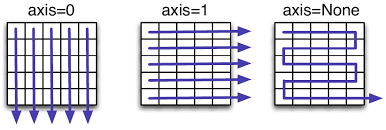
Most of the reduction operations return a scalar. They apply to the array as though it were a list of numbers, regardless of its shape. By specifying the axis parameter, you can apply the “reduction” operation along the specified axis of an array.
axis=0reduces the rows by applying the operation column-by-column.axis=1reduces the columns by applying the operation row-by-row.
col_sum = x.sum(axis=0)
row_sum = x.sum(axis=1)
+---------------+-----------+
|             x | [[1 3 1]  |
|               |  [2 5 1]] |
+---------------+-----------+
| x.sum(axis=0) | [3 8 2]   |
+---------------+-----------+
| x.sum(axis=1) | [5 8]     |
+---------------+-----------+
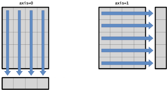
Note that reduction operations change the dimensions of the array: a matrix becomes a vector.
You can keep all the axes of the original array by setting the keepdims parameter to True.
A reduction along
axis=0gives a single-row matrix.A reduction along
axis=1gives a single-column matrix.
col_sum = x.sum(axis=0, keepdims=True)
row_sum = x.sum(axis=1, keepdims=True)
+-------------------------+-----------+   +-------------------------+-----------+
|                       x | [[1 3 1]  |   |                       x | [[1 3 1]  |
|                         |  [2 5 1]] |   |                         |  [2 5 1]] |
+-------------------------+-----------+   +-------------------------+-----------+
|         x.sum(axis = 0) | [3 8 2]   |   |         x.sum(axis = 1) | [5 8]     |
+-------------------------+-----------+   +-------------------------+-----------+
|              shape (1d) | (3,)      |   |              shape (1d) | (2,)      |
+-------------------------+-----------+   +-------------------------+-----------+
| x.sum(0, keepdims=True) | [[3 8 2]] |   | x.sum(1, keepdims=True) | [[5]      |
|                         |           |   |                         |  [8]]     |
+-------------------------+-----------+   +-------------------------+-----------+
|              shape (2d) | (1, 3)    |   |              shape (2d) | (2, 1)    |
+-------------------------+-----------+   +-------------------------+-----------+
1.2.3. Broadcasting#
The term broadcasting describes how NumPy combines arrays with different shapes during arithmetics operations. As mentioned above, operations on two arrays are performed in an element-by-element fashion. In the simplest case, the arrays must have exactly the same shape.
a = np.array([1, 2, 3])
b = np.array([2, 2, 2])

c = a * b
+---+---------+
| a | [1 2 3] |
+---+---------+
| b | [2 2 2] |
+---+---------+
| c | [2 4 6] |
+---+---------+
NumPy’s broadcasting rule relaxes this constraint when the shapes of two arrays meet certain constraints. The simplest example occurs when an array and a scalar value are combined in an arithmetic operation. In this case, the scalar is stretched during the operation, so as to match the shape of the other array.
a = np.array([1,2,3])
b = 2

c = a * b
+---+---------+
| a | [1 2 3] |
+---+---------+
| b | 2       |
+---+---------+
| c | [2 4 6] |
+---+---------+
When operating on two arrays, NumPy compares their shapes element-wise. Subject to certain constraints, the smaller array is “broadcast” across the larger array so that they have compatible shapes. The following are three broadcasting scenarios that often arise in practice.
Scalars broadcast to any array.
Vectors broadcast to matrices with an equal number of columns.
Column matrices broadcast to any vector, and to matrices with an equal number of rows.
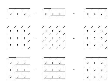
A common beginner mistake in NumPy is to unadvertely perform a binary operation on a single-column matrix and a vector. Due to broadcasting, this produces an unexpected result: each element of the former is combined to every element of the latter, resulting in a matrix of shape equal to the two addends:
vector = np.array([0,1,2])

column = np.array([[0],[1],[2]])

matrix = column + vector
+--------+-----------+
| vector | [0 1 2]   |
+--------+-----------+
| column | [[0]      |
|        |  [1]      |
|        |  [2]]     |
+--------+-----------+
| matrix | [[0 1 2]  |
|        |  [1 2 3]  |
|        |  [2 3 4]] |
+--------+-----------+
In general, broadcasting occurs when the sizes of trailing axes are equal or one. The following are examples of shapes that broadcast.
+------------------------------------+
| A      (2d array):   5 x 4         |
| B      (1d array):       1         |
| Result (2d array):   5 x 4         |
+------------------------------------+
| A      (2d array):   5 x 4         |
| B      (1d array):       4         |
| Result (2d array):   5 x 4         |
+------------------------------------+
| A      (3d array):  15 x 3 x 5     |
| B      (3d array):  15 x 1 x 5     |
| Result (3d array):  15 x 3 x 5     |
+------------------------------------+
| A      (3d array):  15 x 3 x 5     |
| B      (2d array):       3 x 5     |
| Result (3d array):  15 x 3 x 5     |
+------------------------------------+
| A      (3d array):  15 x 3 x 5     |
| B      (2d array):       3 x 1     |
| Result (3d array):  15 x 3 x 5     |
+------------------------------------+
| A      (4d array):   8 x 1 x 6 x 1 |
| B      (3d array):       7 x 1 x 5 |
| Result (4d array):   8 x 7 x 6 x 5 |
+------------------------------------+
Broadcasting fails when the trailing axes are unequal. The following are examples of shapes that do not broadcast.
+--------------------------+
| A (1d array):  3         |
| B (1d array):  4         |
+--------------------------+
| A (1d array):      3     |
| B (2d array):  3 x 4     |
+--------------------------+
| A (2d array):      2 x 1 |
| B (3d array):  8 x 4 x 3 |
+--------------------------+