5.4.7. Convex polyhedron

For a given matrix \(A \in \mathbb{R}^{K \times N}\) and vector \({\bf b} \in \mathbb{R}^K\), the convex polyhedron is a linear constraint defined as

\[ \mathcal{C}_{\rm poly} = \big\{ {\bf w} \in \mathbb{R}^{N} \;|\; A {\bf w} \le {\bf b} \big\}. \]

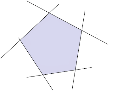
The matrix \(A\) is required to be full rank, and the subset to be nonempty. Depending on how \(A\) and \({\bf b}\) are defined, a polyhedron may be bounded or unbounded. A bounded polyhedron is called polytope, and a 2-dimensional polytope (\(N=2\)) is called polygon. The figure below shows how a polyhedron looks like in \(\mathbb{R}^{2}\) or in \(\mathbb{R}^{3}\).

Polyhedron in 2D

Polyhedron in 3D

5.4.7.1. Constrained optimization

Optimizing a function \(J({\bf w})\) subject to a convex polyhedron can be expressed as

\[ \operatorname*{minimize}_{\textbf{w}\in\mathbb{R}^N}\;\; J({\bf w}) \quad{\rm s.t.}\quad A {\bf w} \le {\bf b}. \]

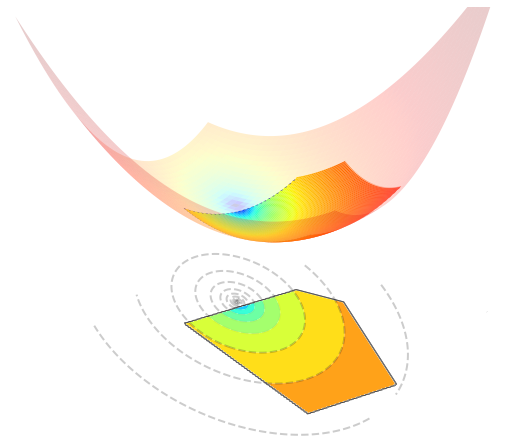
The figure below visualizes such an optimization problem in \(\mathbb{R}^{2}\).

5.4.7.2. Orthogonal projection

The projection of a point \({\bf u}\in\mathbb{R}^{N}\) onto the convex polyhedron is the (unique) solution to the following problem

\[ \operatorname*{minimize}_{{\bf w}\in\mathbb{R}^N}\; \|{\bf w}-{\bf u}\|^2 \quad{\rm s.t.}\quad A{\bf w} \le {\bf b}. \]

The solution can be computed as follows.

Projection onto the polyhedron

\[ \mathcal{P}_{\mathcal{C}_{\rm poly}}({\bf u}) = {\bf u} - A^\top {\bf c}^* \]

The vector \({\bf c}^* \in \mathbb{R}^K\) is the unique minimizer to the non-negative least squares problem

\[ \operatorname*{minimize}_{{\bf c}\in \mathbb{R}^K}\;\; \frac{1}{2} \|A^\top {\bf c} - {\bf u}\|^2 + {\bf c}^\top {\bf b} \quad{\rm s.t.}\quad {\bf c}\ge 0. \]

Although there exists no closed-form formula for the optimal \({\bf c}^*\), it can be effectively computed by numerical methods.

5.4.7.3. Implementation

In the following implementation, the dual problem is solved with an algorithm called FISTA, whose iterations are reported here after. This solution is suitable only for polyhedra with small \(N\) and \(K\). A faster and more scalable implementation is based on the projected Newton method proposed by Dimitri Bertsekas in 1982.

\[\begin{split} \begin{aligned} &L = {\rm sup}_{{\bf c}}\|\nabla^2 f({\bf c})\|_2\\ &{\bf c}_0 = {\bf y}_0 = {\bf 0} \\ &\textrm{For $i=0, 1, \dots$}\\ &\left\lfloor \begin{aligned} {\bf y}_{i+1} &= \mathcal{P}_{\mathcal{C}}\big({\bf c}_i - \frac{1}{L} \nabla f({\bf c}_i)\big) \\ {\bf c}_{i+1} &= {\bf y}_{i+1} + \frac{i}{i+3} \big({\bf y}_{i+1} - {\bf y}_{i}\big) \end{aligned} \right. \end{aligned} \end{split}\]

def project_poly(u, A, b):
    assert A.ndim == 2, "'A' must be a matrix (2 axes)"
    assert b.ndim == 1, "'b' must be a vector (1 axis)" 
    assert A.shape[0] == b.shape[0], "The size of 'b' must be equal to the number of rows of 'A'"
    assert np.linalg.matrix_rank(A) == np.min(A.shape), "'A' must have full rank"
    
    def nnls(epochs=1000):
        y = 0
        c = np.zeros_like(b)
        step = 1 / np.linalg.norm(A, ord=2)**2
        for i in range(epochs):
            yo= y
            g = A @ (A.T @ c - u) + b
            y = np.maximum(0, c - step * g)
            c = y + i/(i+3) * (y - yo)
        return c
    
    c = nnls()
    p = u - A.T @ c
    
    return p

Here is an example of use.

u = np.array([1.5, -2])

A = np.array([[-1, -2],
              [-2, -1],
              [ 1, -1]])
b = np.array([0, 0, 3])

p = project_poly(u, A, b)

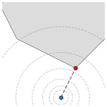
The next figure visualizes a point \({\bf u}\in \mathbb{R}^{2}\) (blue dot) along with its projection (red dot) onto this set.

5.4.7.4. Proof

By using the Lagrange multipliers to remove inequality constraints, the projection onto the convex polyhedron is the (unique) solution to the following problem

\[ \operatorname*{minimize}_{{\bf w}\in\mathbb{R}^N}\;\sup_{{\bf c}\ge0}\; \frac{1}{2} \|{\bf w}-{\bf u}\|^2 + {\bf c}^\top (A{\bf w} - {\bf b}). \]

Strong duality holds, because this is a convex problem with linear constraints. Hence, it can be equivalently rewritten as

\[ \operatorname*{maximize}_{{\bf c}\ge0}\;\inf_{{\bf w}\in\mathbb{R}^N}\; \frac{1}{2} \|{\bf w}-{\bf u}\|^2 + {\bf c}^\top (A{\bf w} - {\bf b}). \]

Setting to zero the gradient w.r.t. \({\bf w}\), the inner minimization is solved by

\[ {\bf w}^* = {\bf u} - A^\top {\bf c}, \]

Replacing \({\bf w}^*\) in the criterion yields

\[\begin{split} \begin{aligned} \frac{1}{2} \|{\bf w}^*-{\bf u}\|^2 + {\bf c}^\top (A{\bf w}^* - {\bf b}) &= \frac{1}{2} \|{\bf u} - A^\top {\bf c}-{\bf u}\|^2 + {\bf c}^\top (A{\bf u} - AA^\top {\bf c} - {\bf b}) \\ &= \frac{1}{2} \|A^\top {\bf c}\|^2 + {\bf c}^\top A{\bf u} - \|A^\top {\bf c}\|^2 - {\bf c}^\top {\bf b} \\ &= -\frac{1}{2} \|A^\top {\bf c}\|^2 + {\bf c}^\top A{\bf u} - {\bf c}^\top {\bf b} \\ &= -\frac{1}{2} \|A^\top {\bf c} - {\bf u}\|^2 - {\bf c}^\top {\bf b}. \end{aligned} \end{split}\]

Hence, the outer maximization is equivalent to

\[ \operatorname*{minimize}_{{\bf c}\ge0}\; \frac{1}{2} \|A^\top {\bf c} - {\bf u}\|^2 + {\bf c}^\top {\bf b}. \]

This is a non-negative least squares problem that can be efficiently solved with numerical methods.