5.7.2. Example 7#
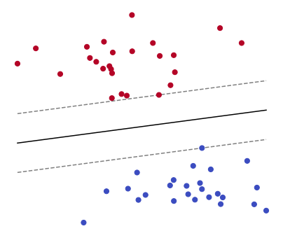
Look at the points shown in the figure below. Notice how they can be divided into two groups by a straight line. Given such “linearly separable” points and their respective groups, how do you find the line that perfectly divides them? The answer is to formulate this task as an optimization problem.
5.7.2.1. Formulation#
Remember that a line can be represented by the equation
More precisely, the solutions \((x,y)\) of the above equation form a line, whose slope and intercept are governed by the coefficients \((w_0, w_1, w_2)\). A linear equation is homogeneous, meaning that its coefficients can be multiplied by any constant \(c\ne0\) without changing the line it represents, namely
If \(w_2\neq0\), the linear equation implicitly defines the variable \(y\) as a function of the variable \(x\), yielding
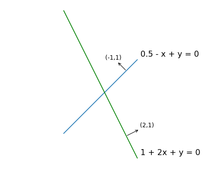
The graph of this function is a line with slope \(-\frac{w_1}{w_2}\) and intercept \(- \frac{w_0}{w_2}\). Remark that the slope depends only on coefficients \(w_1\) and \(w_2\), but not \(w_0\). In fact, the vector \((w_1, w_2)\) is orthogonal to all the (parallel) lines with slope \(- \frac{w_1}{w_2}\). The proof consists of taking two points \((x_0', y_0')\) and \((x_0'', y_0'')\) on the line \(w_0 + w_1 x + w_2 y = 0\), and noting that the scalar product between the vectors \((x_0'-x_0'', y_0'-y_0'')\) and \((w_1, w_2)\) is trivially equal to zero. See the figure below.
5.7.2.1.1. Separating line#
Consider two sets of points that can be separated by a straight line. They are denoted as
The goal is to find a line that actually separates them. Intuitively, the desired line must be placed so that every point in the set \(\mathcal{S}^+\) lies on the “upper” side of the line, and each point in the set \(\mathcal{S}^-\) lies on the “lower” side. This requirement can be mathematically expressed by a series of linear inequalities
Strict inequalities are problematic in constrained optimization, and they should always be avoided. Luckily in this case, the condition that a value must be strictly positive can be equivalently enforced by requiring that such value should not be lower than a positive constant \(a>0\). A similar reasoning applies to a strictly negative value, which should not be higher than a negative constant \(-a\). As linear inequalities are positively homogeneous, the choice \(a=1\) can be made without loss of generality. Then it follows that the above linear inequalities are equivalent to
The figure below illustrates the geometry of these constraints. For a given triplet \((w_0, w_1, w_2)\) appearing in the title, the region delimited by the dashed lines is highlighted either in green or magenta. The green indicates that the triplet satisfies all the linear inequalities. This happens when all the red points are “on or above” the upper parallel line, and all the blue points are “on or below” the lower parallel line. Interact with the slider to multiply the coefficients by a smaller or larger constant. These are just a few examples among the infinitely many triplets that could satisfy or violate the constraints.
Note
The coefficients \((w_0, w_1, w_2)\) determine the separating line \(\,w_0 + w_1 x + w_2 y = 0\).
The upper parallel line \(\,w_0 + w_1 x + w_2 y = 1\,\) is shifted above the separating line.
The lower parallel line \(\,w_0 + w_1 x + w_2 y = -1\,\) is shifted below the separating line.
The separating line passes evenly through the region delimited by the upper and lower parallel lines.
A triplet \((w_0, w_1, w_2)\) satisfies the constraints if and only if there are no points inside the region delimited by the upper and lower parallel lines.
Multiplying the coefficients \((w_0, w_1, w_2)\) by a constant modifies the distance between the upper and lower parallel lines, but does not change the separating line.
Changing the coefficients \((w_0, w_1, w_2)\) individually alters the slope or the intercept of the separating line.
5.7.2.1.2. Maximum margin#
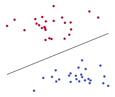
Finding the line that splits two distinct groups of points is an ill-posed problem, because infinitely many lines could be drawn to perfectly separate the data. The figure below shows two such lines. Given that both lines would perfectly split the data, which one could be considered the “best”? A reasonable criterion for judging the quality of a separating line is via the margin, that is the distance between the upper and lower parallel lines. The larger the margin is, the better the associated line separates the points. In the figure below, the black line has a larger margin than the green line, thus it can be considered as a better separating line.
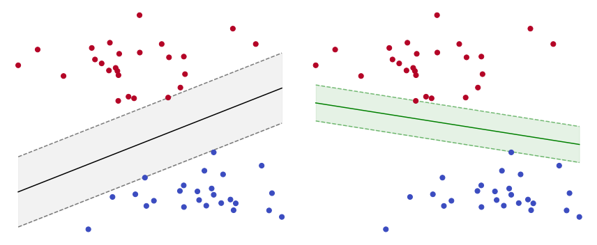
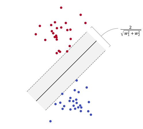
The separation by maximum margin boils down to finding the coefficients \((w_0, w_1, w_2)\) such that the parallel lines \(w_0 + w_1 x + w_2 y = \pm 1\) have the largest possible distance. It can be proved that the distance between such lines is equal to
Therefore, the separating line with the smallest possible normal vector \((w_1, w_2)\) is the one that does so by maximum margin. This fact is illustrated in the figure below.
Proof
Let \((x',y')\) be a point on the upper parallel line, and let \((x'',y'')\) be a point on the lower parallel line. It follows that
Further assume the vector \((x'-x'', y'-y'')\) is orthogonal to the separating line, so that its norm measures the distance between the upper and lower parallel lines. Then, such vector is parallel to the normal vector \((w_1,w_2)\), and their scalar product is equal to the product of their norm, namely
Putting all together, the distance between the parallel lines is equal to
5.7.2.2. Optimization problem#
Finding the separating line with maximum margin can be formulated as a constrained optimization problem. It amounts to minimizing the squared norm of the normal vector \((w_1,w_2)\) subject to a series of linear inequalities. This yields
Note that the variable \(w_0\) does not appear in the function to minimize (so this is not an orthogonal projection).
5.7.2.2.1. Feasible set#
The problem is constrained by \(M^{+} + M^{-}\) linear inequalities, so the feasible set is a convex polyhedron. Recall that a convex polyhedron can be generically expressed as the set of inequalities \(A{\bf w} \le {\bf b}\). This abbreviated notation can be specialized to the above problem by defining the matrix \(A\) and the vector \({\bf b}\) as follows
With the notation just introduced, the problem can equivalently formulated as
It is now apparent that the problem can be solved through projected gradient descent.
Convex polyhedron
The equivalence between the convex polyhedron defined above and the constraints of the problem is shown below.
5.7.2.2.2. Projection onto the feasible set#
Solving a problem with projected gradient descent requires to implement the orthogonal projection onto the feasible set. In this case, the feasible set is a convex polyhedron \(\mathcal{C}_{\rm poly} = \{ {\bf w} \in \mathbb{R}^{N} \;|\; A {\bf w} \le {\bf b}\}\). The projection of a point \({\bf u}\) onto a polyhedron is equal to
where \(\bar{\bf c} \in \mathbb{R}^K\) is the unique minimizer to the non-negative least squares problem
Although there exists no closed-form formula for the optimal \(\bar{\bf c}\), it can be effectively computed by numerical methods. More details can be found in the section discussing the projection onto a convex polyhedron.
5.7.2.3. Numerical resolution#
Projected gradient descent allows you to numerically solve an optimization problem in three steps:
implement the cost function with NumPy operations supported by Autograd,
implement the projection onto the feasible set,
select the initial point, the step-size, and the number of iterations.
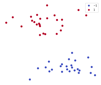
Before going any further, it is helpful to make the problem more concrete. The code below generates a random bunch of points. The matrix points stacks all the points \((x,y)\), whereas the vector labels holds a number for each point. The value labels[i] is either \(+1\) or \(-1\) for indicating the group to which it belongs the point points[i].
from sklearn.datasets import make_blobs

points, labels = make_blobs(n_samples=50, centers=2, random_state=10, cluster_std=2)

points /= points.max(axis=0)      # each row is a point (x,y) normalized

labels = 2 * labels[:,None] - 1   # each point is tagged +1 or -1
5.7.2.3.1. Cost function#
Let’s start by implementing the cost function. Nothing special here. Its implementation is a Python function that takes a vector w of length 3, where the element w[0] holds the value \(w_0\), the element w[1] holds the value \(w_1\), and so forth. The only caveat is that the cost function sums the squares of all variables except \(w_0\).
cost_fun = lambda w: np.sum(w[1:]**2)
5.7.2.3.2. Orthogonal projection#
With the cost function out of the way, let’s move on to implement the projection. The cell below implements a solution that is suitable for polyhedra with small \(N\) and \(K\). More details can be found in the section discussing the projection onto a convex polyhedron.
def project_poly(u, A, b):

    assert np.linalg.matrix_rank(A) == np.min(A.shape), "The matrix must have full rank"

    def nnls(epochs=1000):
        y = 0
        c = np.zeros_like(b)
        step = 1 / np.linalg.norm(A, ord=2)**2
        for i in range(epochs):
            yo= y
            g = A @ (A.T @ c - u) + b
            y = np.maximum(0, c - step * g)
            c = y + i/(i+3) * (y - yo)
        return c

    c = nnls()
    p = u - A.T @ c

    return p
The function project_poly expects three arguments: the point \({\bf u}\) to be projected, as well as the matrix \(A\) and the vector \(b\) that define the polyhedron. In the cell below, the matrix \(A\) and the vector \({\bf b}\) are created according to the problem specifications. A small extract of the result is shown right after.
A = np.hstack([labels, points * labels])

b = - np.ones(points.shape[0])
===== A[:5] =====
[[ 1.         -0.04093607  0.62728693]
 [ 1.          0.20353536  0.52013473]
 [-1.         -0.4546765   1.00998615]
 [ 1.          0.06940629  0.3410282 ]
 [-1.         -0.677963    1.06314613]]

===== b[:5] =====
[-1. -1. -1. -1. -1.]
Remember that the projection must be implemented as a Python function that takes one vector, and returns another vector of the same size. No other input or output is allowed. So the function project_poly cannot be used directly, because it expects the three arguments u, A and b. The workaround is to define a new “wrapper” function that takes a single input, and whose only job is to call project_poly using predefined inputs for all the arguments that will not change during the optimization process. This is precisely what the function below does: it sets the arguments A and b to the array created just above. It is such function (and not directly project_poly) that will be then given to the optimization algorithm.
projection = lambda u: project_poly(u, A, b)
5.7.2.3.3. Execution#
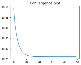
Now it remains to set an initial point, the step-size, the number of iterations, and then run projected gradient descent.
init = np.zeros(3)  # initial point
alpha = 0.1         # step-size
epochs = 50         # number of iterations

w, history = gradient_descent(cost_fun, init, alpha, epochs, projection)
The figure below shows the separating line defined by the optimal solution \(\bar{\bf w} = (\bar{w}_0, \bar{w}_1, \bar{w}_2)\).