Maximum curvature#
In addition to the trial and error approach, there are mathematical tools to choose a step-size that guarantees the convergence of gradient descent. These strategies are often conservative or computationally expensive, depending on the function being minimized. Nonetheless, they always provide solutions that work “out of the box” in almost all situations. In the following, we will focus on the conservatively optimal step-size defined by the Lipschitz constant of the gradient.
Quadratic approximation#
Crucial to our analysis is the following symmetric quadratic function (with \(\alpha>0\)):
Notice what precisely this is. The first two terms on the right-hand side constitute the formula for the hyperplane tangent to \(J(\mathbf{w})\) at a point \(\mathbf{w}_k\). The final term is a simple quadratic function that turns the tangent hyperplane into a convex and perfectly symmetric parabola, whose curvature is controlled in every dimension by the parameter \(\alpha\). This parabola is still coincident to the function \(J(\mathbf{w})\) at \(\mathbf{w}_k\), matching both the function and derivative values at this point.
The figure below plots the function \(J(w) = \text{cos}(w + 2.5) + 0.1w^2\), its tangent line (green) at a point \(w_k\) (red dot), and its quadratic approximation \(Q_{\alpha}\left(w\,|\,w_k\right)\) (blue) at \(w_k\) with a fixed \(\alpha\).
Gradient descent revisited#
The beauty of such simple quadratic approximation is that we can easily compute a unique global minimum for it, regardless of the curvature \(\alpha\), by checking the first order optimality condition. Setting its gradient to zero we have
Rearranging the above and solving for \(\mathbf{w}\), we can find the minimizer of \(Q_{\alpha}({\bf w},{\bf w_k})\), which we call \(\mathbf{w}_{k+1}\), and is given by
The minimum of our simple quadratic approximation is precisely a gradient descent step at \(\mathbf{w}_k\) with step-size \(\alpha\). This yields an alternative perspective on gradient descent. We can now see it as an algorithm that uses a simple quadratic approximation to move towards a minimum, namely
This idea is illustrated below for the function \(J(w) = \text{cos}(w + 2.5) + 0.1w^2\). Moving the slider animates each step of the gradient descent process, as well as both the tangent line and quadratic approximations driving each step.
Step-size revisited#
Carefully choosing the step-size is important to ensure the convergence of gradient descent. The actual “proper choice” however depends on the function being minimized. A possible solution to tackle this issue is the following.
Tip
Choose the step-size \(\alpha>0\) small enough to make the function decrease at each step of gradient descent.
Our alternative perspective tells us that in making the step-size \(\alpha\) small, we are narrowing the associated quadratic approximation (i.e., increasing its curvature), whose minimum is the point that gradient descent will move to in a single step. As a rule of thumb, the step-size \(\alpha\) should be decreased until the minimum value of the quadratic approximation lies above the cost function. By doing so, we are guaranteed to decrease the function value with a single step of gradient descent, so that \(J({\bf w}_{k+1})< J({\bf w}_k)\) whenever \(\nabla J({\bf w}_k) \neq {\bf 0}\). This fact can be summarized in the sufficient descent condition.
Descent condition (sufficient)
This idea is shown below for the function \(J(w) = \text{cos}(w + 2.5) + 0.1w^2\). Moving the slider increases the step-size, making the quadratic approximation larger and larger. A decrease \(J\left(\mathbf{w}_{k+1}\right) < J\left(\mathbf{w}_{k}\right)\) is ensured by all values of \(\alpha\) such that \(J\left(\mathbf{w}_{k+1}\right) \le Q_{\alpha}\left(\mathbf{w}_{k+1}\,|\,\mathbf{w}_{k}\right)\), which visually consists of keeping the blue cross above the greed dot. In this particular example, however, you can notice that a decrease also occurs for some step-sizes not respecting the above condition. This happens because the latter is a sufficient but not necessary condition for decreasing the function \(J\left(\mathbf{w}\right)\) at each iteration.
Quadratic majorant#
How can we set the step-size \(\alpha\) such that the minimum value of the quadratic approximation lies above the cost function? We can choose the value that reflects the greatest amount of curvature in the cost function. Such value indeed yields the widest quadratic approximation that lies completely above the function at every point of tangency. In other terms, when the curvature of \(J({\bf w})\) is upper bounded, it is possible to choose the step-size \(\alpha\) such that \(Q_{\alpha}\left(\mathbf{w}\,|\,\mathbf{p}\right)\) is a majorant of \(J({\bf w})\) for every \({\bf p}\). This result can be summarized as follows.
Descent lemma
The above result becomes an equivalence when \(J\) is convex.
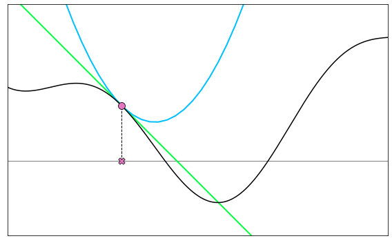
The idea is illustrated below for the function \(J(w) = \text{sin}(3w) + 0.1w^2 + 1.5\). Use the slider to move the current point (marked as a red dot). At each point, the quadratic approximation (shown in light blue) is made with \(\alpha\) equal to the maximum curvature of \(J(w)\). This ensures that the quadratic approximation always lies completely above the function, including its minimum (marked with a green dot). The evaluation of this minimum by the function and quadratic approximation are marked with green and dark blue dots, respectively. Notice how at every point of the function domain (except stationary points), the gradient descent step given by the minimum of this quadratic approximation always leads to a smaller value of the function. In other words, the red dot is always higher on the function than the green one.
Lipschitz constant#
The curvature of a twice-differentiable function is expressed by the second derivative. Specifically, the maximum curvature of a one-dimensional function is the largest absolute value of the second derivative, provided that such value exists
Likewise, the maximum curvature of a multi-dimensional function is the largest absolute eigenvalue of the Hessian matrix
Since every function with bounded curvature has Lipschitz continuous gradient, the maximum curvature \(L\) is also called the Lipschitz constant of the gradient. As daunting a task as this may seem, the Lipschitz constant can be computed analytically for a range of common functions. Note however that not all the functions have an upper bound on their curvature. One such example is the function \(e^w\), whose first derivative is not Lipschitz continous. So, for the functions with bounded curvature, the Lipschitz constant gives the following choice of step-size.
Conservative step-size
With the step-size equal to the reciprocal of the maximum curvature, gradient descent is guaranteed to converge to a stationary point, because we know for sure that the minimum value of the quadratic majorant \(Q_{1/L}\left(\mathbf{w}\,|\,\mathbf{w}_k\right)\) always lies above the cost function \(J(\mathbf{w})\) for every point of tangency \(\mathbf{w}_k\), ensuring a decrease in the function value at each step of gradient descent.
The figure below plots the function \(J(w) = \log\left(1+e^{2w-10}\right) + 5\log\left(1+e^{-w}\right)\) and its second derivative. You can see that \(J''(w)\) is upper bounded by the constant \(L=5/4\). Hence, the first derivative is Lipschitz continuous, which intuitively means that \(J'(w)\) is limited in how fast it can change, or equivalently that the function \(J(w)\) has bounded curvature.
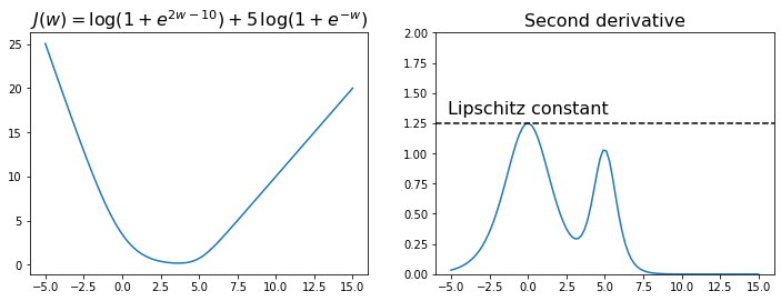
The choice of step-size \(\alpha = \frac{1}{L} = 4/5\) guarantees that every step of gradient descent decreases the function value. This is illustrated in the animation below, where the red dot marks a generic point \(w_k\), and the green dot marks the point generated with a step of gradient descent as \(w_{k+1} = w_k - \frac{1}{L} J'(w_k)\).
Examples#
Let us compute the Lipschitz constant of the function
The second derivative of this function is
whose maximum yields the Lipschitz constant
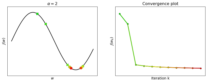
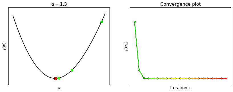
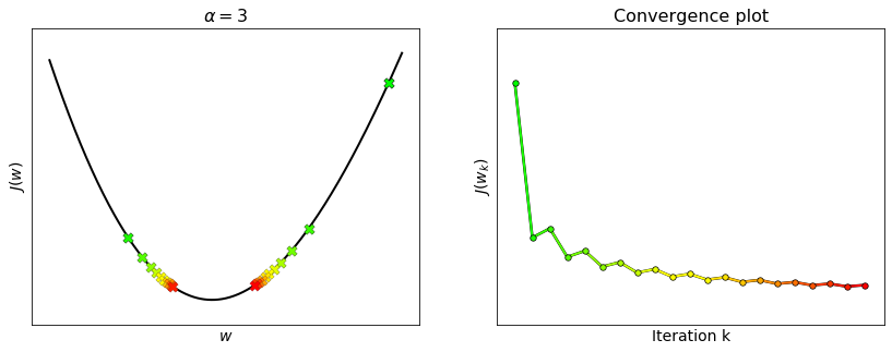
Runnnig gradient descent with \(\alpha = \frac{1}{L}\) ensures the convergence, but it is not guaranteed for higher values.
Let us compute the Lipschitz constant of the function
The second derivative of this function is
whose maximum leads to the Lipschitz constant:
Runnnig gradient descent with \(\alpha = \frac{1}{L}\) ensures the convergence, but it is not guaranteed with higher values.
Let us compute the Lipschitz constant of the function
The Hessian matrix of this function is
whose maximum eigenvalue yields the Lipschitz constant:
Runnnig gradient descent with \(\alpha = \frac{1}{L}\) ensures the convergence, but it is not guaranteed with higher values.
Limitations#
Choosing \(\alpha=\frac{1}{L}\) is sufficient to ensure the convergence of gradient descent with Lipschitz-differentiable functions. However, the constant \(L\) only captures the maximum curvature of a function, and ignores any local variation of the function’s curvature that may occur in other parts of its domain. A step-size equal to the reciprocal of the maximum curvature could then be smaller than necessary, especially if the maximum curvature is situated far away from the minimum. This is why such step-size is deemed as “too conservative”. Gradient descent may still converge with a larger step-size, although it is no longer ensured that the value of the cost function will decrease at each iteration.
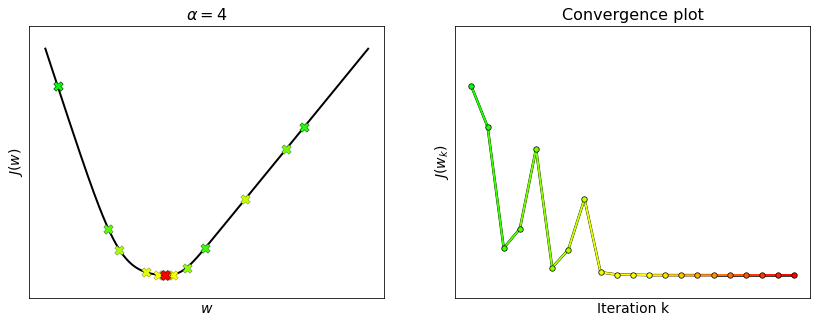
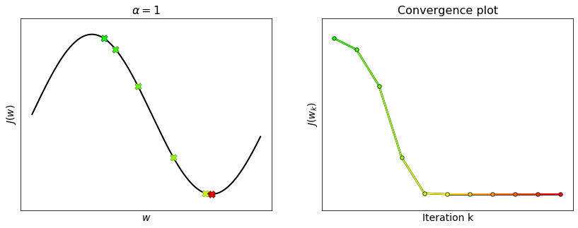
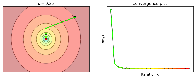
For example, consider the function \(J(w) = \log\left(1+e^{2w-10}\right) + 5\log\left(1+e^{-w}\right)\). The second derivative takes its maximum at \(L=1.25\) (see the plot above), but the choice \(\alpha=1/L = 0.8\) is too conservative. This happens because the local curvature around the minimum is much smaller than \(L\). Hence, gradient descent is able to converge with step-sizes well beyond the theoretical limit. See the example below with \(L_{\rm local}\approx 0.25\) and \(\alpha=1/L_{\rm local}=4\). As large step-sizes may lead to a faster convergence, many strategies have been developed to “locally adapt” the step-size. Some techniques such as scheduling, line search and backtracking will be discussed in the next sections.