2.5. Local optimization#
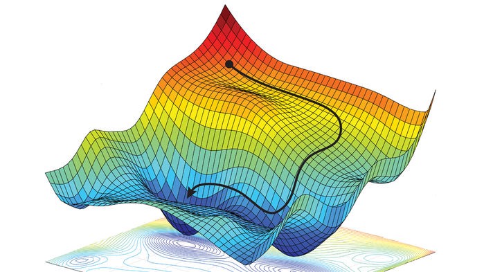
Grid search works by probing a multitude of uncorrelated points to find an approximate minimum of a function. This is however just one way to solve an optimization problem. Other approaches are based on local optimization, where a single point is progressively refined by pulling it toward lower and lower values of the cost function, until a global or local minimum is reached. This progressive refinement can be designed to be extremely effective, making it more scalable than grid search.
2.5.1. Sequential refinement#
A generic sequential refinement scheme works as follows. Initially, a starting point \({\bf w}_0\) is selected, randomly or in any other way. Then, a “descent direction” at \({\bf w}_0\) is found. This is a vector \({\bf d}_0\) pointing in such a direction as to decrease the value taken by the function \(J({\bf w})\) at the point \({\bf w}_0\). By doing so, the first update can be literally computed as \({\bf w}_1 = {\bf w}_0 + {\bf d}_0\). Thereafter, a new descent direction \({\bf d}_1\) is found at \({\bf w}_1\), so as to compute the second update \({\bf w}_2 = {\bf w}_1 + {\bf d}_1\). This process is repeated several times, producing the following sequence of points:
Here, it is importat that the descent directions are selected so as to generate a decreasing sequence
There are numerous ways of determining proper descent directions, which distinguish local optimization methods from each other. In this section, we will discuss one specific strategy in more detail, called random search.
2.5.2. Random search#
The laziest strategy to find a descent direction consists of looking around in random directions, until a point lower on the function is found. This amounts to continuously updating a point \({\bf w}_{k}\) and a step-size \(\alpha_k\) through the following steps.
Determine a set of random directions \({\bf d}_{k}^{(1)},\dots,{\bf d}_{k}^{(S)}\).
Compute the update \({\bf \bar{w}}_{k+1}^{(s)} = {\bf w}_{k}+\alpha_k \,{\bf d}_k^{(s)}\) for every direction \(s\in\{1,\dots,S\}\).
Choose the point \({\bf \bar{w}}_{k+1}^{(s^*)}\) with the smallest value among \(J({\bf \bar{w}}_{k+1}^{(1)}), \dots, J({\bf \bar{w}}_{k+1}^{(S)})\).
Set \({\bf w}_{k+1} = {\bf \bar{w}}_{k+1}^{(s^*)}\) if it attains a lower value than \({\bf w}_{k}\) on the function.
Adjust the step-size \(\alpha_{k+1}\) and repeat the process.
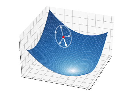
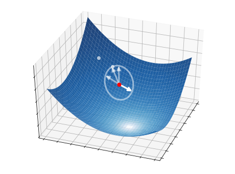
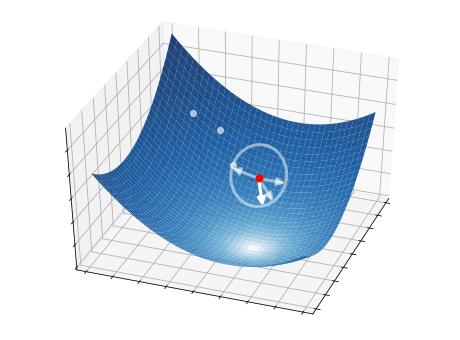
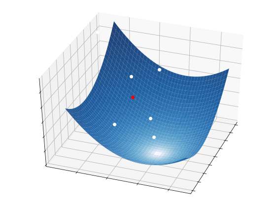
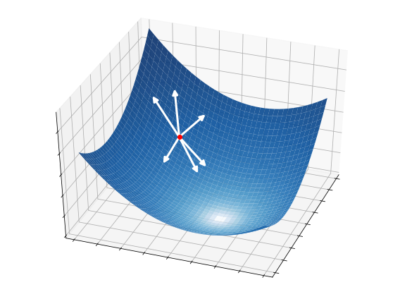
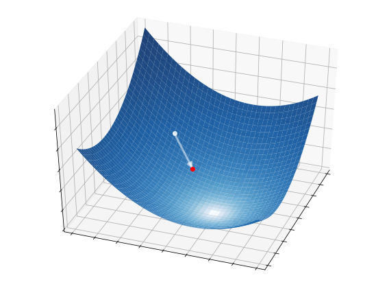
This idea is illustrated in the pictures below on a two-dimensional function. At each iteration, \(S=4\) candidate directions (white arrows) are randomly sampled, and the best one is selected as a descent direction (strong white arrow). The latter is then used to update the current point (red circle), from which the process starts over.

2.5.2.1. Step 1 - Directions#
How do we choose a set of random directions at the \(k\)-th iteration? We can draw vectors from a normal distribution with zero mean and unitary variance:
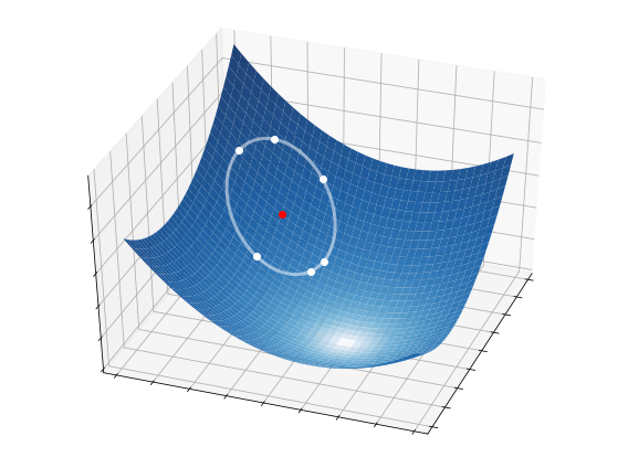
The only issue with doing so is that each candidate direction would have different length. We overcome this issue by normalizing them to have unitary length:
This ensures that the random directions are sampled from a circonference with unitary radius centered at \({\bf w}_{k}\).
2.5.2.2. Step 2 - Selection#
Once the candidate directions are selected, they are scaled by the step-size \(\alpha_k\) to completely control how far we travel along a given direction. Then, we test all the candidate directions and take the one providing the greatest decrease on the function:

2.5.2.3. Step 3 - Update#
With the selected direction, we perform a tentative update
We make \({\bf \bar{w}}_{k+1}\) as a new point only if it decreases the function, otherwise we discard it and start over:
2.5.2.4. Step 4 - Step-size#
The step-size \(\alpha_k\) is a positive value that controls the distance travelled at each iteration, in the sense that
The choice of step-size is essential to guarantee that the sequence \({\bf w}_0,{\bf w}_1,\dots,{\bf w}_k\) converges to a (global or local) minimum of the function. While it may be tempting to select a constant step-size, this approach only works with sufficiently small values, at the expense of requiring many iterations before arriving at convergence. Even so, the algorithm can only get so close to a solution, because the update on the current point cannot be smaller than the step-size itself.
A better approach consists of adapting the step-size as the algorithm goes. The 1/5-th success rule is one of the oldest strategies designed for this purpose. It consists of increasing the step-size after a successful step and decreasing it after a failure, so as to keep a success probability of 1/5. Concretely, the step-size is updated at the end of each iteration as follows
The 1/5-th success rule ensures that \(\alpha_k\to0\) as \(k\to+\infty\), so the algorithm eventually stops (most likely at a global or local minimum). Note that the factor 1.5 may be replaced with any value strictly greater than one.
2.5.3. Numerical implementation#
The following is a Python implementation of random search. Each step of the algorithm is translated into one or several lines of code. Numpy library is used to vectorize operations whenever possible.
def random_search(cost_fun, init, alpha, epochs, n_points, factor=1.5):
    """
    Finds the minimum of a function.

    Arguments:
    cost_fun -- cost function | callable that takes 'w' and returns 'J(w)'
    init     -- initial point | vector of shape (N,)
    alpha    -- step-size     | scalar
    epochs   -- n. iterations | integer
    n_points -- n. directions | integer
    factor   -- step adjuster | scalar greater than 1

    Returns:
    w -- minimum point | vector of shape (N,)
    """
    assert factor > 1, "The factor must be greater than one"

    # Initialization
    w = np.array(init).ravel()  # vector (1d array)
    J = cost_fun(w)

    # Refinement loop
    for k in range(epochs):

        # Step 1. Choose random directions
        directions  = np.random.randn(n_points, w.size)
        directions /= np.linalg.norm(directions, axis=1, keepdims=True)

        # Step 2. Select the best direction
        w_all = w + alpha * directions
        costs = [cost_fun(wk) for wk in w_all]
        i_min = np.argmin(costs)

        # Steps 3 & 4. Update point and step-size
        if costs[i_min] < J:
            w = w_all[i_min]
            J = costs[i_min]
            alpha *= factor
        else:
            alpha /= factor**0.25

    return w
The python implementation requires five arguments:
the function to optimize,
a starting point,
the initial step-size that controls the distance travelled at each iteration,
the number of iterations to be performed,
the number of directions to test per iteration.
An usage example is presented next.
# cost function of two variables
cost_fun = lambda w: (2*w[0]+1)**2 + (w[1]+2)**2

init = [1, 3]  # starting point
alpha  = 0.01  # initial step-size
epochs = 20    # number of iterations
n_points = 10  # number of directions per iteration

# numerical optimization
w = random_search(cost_fun, init, alpha, epochs, n_points)
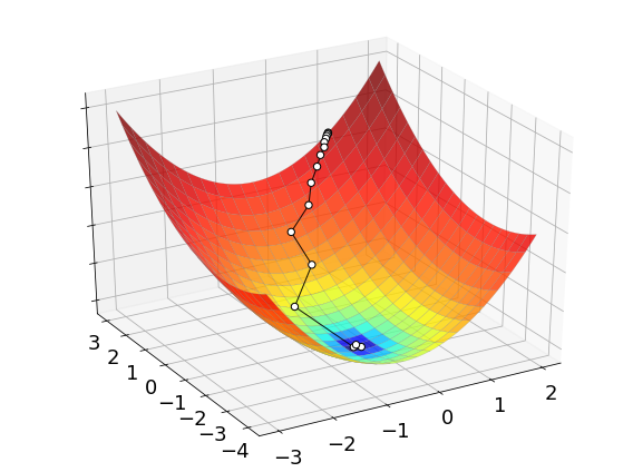
The process of optimizing a function with random search is illustrated below. The white dots mark the sequence of points generated by the algorithm to find its final approximation of the minimum. While these points may seem to be much less than grid search, keep in mind that random search tests a bunch of directions at each iteration. These directions are not shown in the picture, but they definitely contribute to the overall complexity of the method.
2.5.4. Curse of dimensionality#
Random search is also crippled by the curse of dimensionality, although this phenomenon is a bit less severe. The issue here is that the chance of randomly selecting a descent direction gets lower and lower as the dimension \(N\) of the cost function increases. For instance, the descent probability falls below \(1\%\) when \(N=30\). Another big issue with random search lies in the highly inefficient way in which descent directions are found. If we had a computationally cheaper way of finding descent directions, then the local method paradigm would work extremely well. This is precisely what we will do in later chapters, which are dedicated solely to the pursuit of finding good and computationally cheap descent directions, leading to a powerful algorithm called gradient descent.